`
ε
-Regularized Economic Model Predictive Control for Thermal Comfort
in Multizone Buildings
Farah Gabsi
1,2
, Frederic Hamelin
1
, Nathalie Sauer
2
and Joseph J. Yame
1
1
Centre de Recherche en Automatique de Nancy, University of Lorraine, Vandoeuvre-les-Nancy, France
2
Laboratoire de G
´
enie Informatique, de Production et de Maintenance, University of Lorraine, Metz, France
Keywords:
Energy-efficient Buildings, Model Predictive Control, Regularization.
Abstract:
This paper presents a new thermal regulation technique for multizone buildings, possibly equipped with dis-
continuously (on/off) operating HVAC actuators, based on regularized economic model predictive control
(REMPC). In the presence of actuators operating on an on/off basis, it often happens that the control scenario
resulting from such a strategy is very “aggressive” towards these same actuators due to the many on/off cycles.
This phenomenon can lead to premature wear of the actuators most sensitive to these repeated state changes
(especially heat pump compressors). In order to take into account the “aggressiveness” of a control scenario
and to increase the lifetime of the actuators, an economic criterion with a regularization term based on the
parsimony-promoting property of the `
ε
-norm (ε small) is used. This term is sufficiently generic to allow the
regularization of the optimal control law by taking into account discontinuous control inputs (on/off), reducing
the number of actuators used at any given time or avoiding inappropriate control scenarios (alternating use of
heat pump in heating/cooling modes,...). To solve the minimization problem of the non-convex `
ε
-regularized
economic criterion, we use an iterative algorithm recently derived in (Gabsi et al., 2018b). The effectiveness
of the proposed control strategy is illustrated on the “Eco-Safe” platform at CRAN Nancy, France.
1 INTRODUCTION
In the context of intelligent buildings, modern cen-
tralised automation systems are often used to im-
prove their energy efficiency. “Building Automation
and Control Systems” (BACS) are generally based
on a dynamic model of buildings. Depending on
their complexity and/or performance, they may also
include a precise description of the most energy-
intensive equipment (heating, ventilation and air con-
ditioning (HVAC) systems (Rawlings et al., 2018),...),
the price of electricity or the behaviour of occupants.
In addition to this optimized energy management,
thermal comfort inside the building is usually a fac-
tor taken into consideration, which leads to a global
control problem (Gabsi et al., 2018b).
Model Predictive Control (MPC) is one of the
most used advanced control strategies in this context,
mainly due to its ability to achieve economic objec-
tives, taking into account a simplified dynamic model
and different constraints (Godina et al., 2018), (Serale
et al., 2018). The modelling method influences the
actual practice of MPC in buildings because of its
cost and scalability (Gabsi et al., 2017), (Gabsi et al.,
2018a), (Zhuang et al., 2018). Economic Model Pre-
dictive Control (EMPC) (Zong et al., 2017), (Rawl-
ings et al., 2018), (Ellis et al., 2014) is becoming in-
creasingly popular because of its interest in consider-
ing more general economic cost functions than tradi-
tional quadratic cost functions.
In recent years, the theory of LASSO (Least Ab-
solute Selection and Shrinkage Operator), particu-
larly used in signal processing, has led to the emer-
gence of new predictive control strategies called “`
asso
MPC” (Gallieri and Maciejowski, 2012), (Rao, 2018)
or RMPC for “Regularized MPC” (Amy et al., 2016).
By using penalty criteria in `
1
-norm that favor some
kinds of sparse controls, it becomes possible, for ex-
ample, to limit the number of active control inputs in
an over-actuated system (Gallieri and Maciejowski,
2015) or to prioritize actuator actions and efficiently
distribute control effort (Amy et al., 2016). It is
also possible to consider certain control applications
that require the use of piecewise constant or impulse-
type control signals, with as few changes as possible
(Pakazad et al., 2013). In the same way, a binary reg-
ularization term can be introduced in order to penalize
differently the power variations of actuators depend-
Gabsi, F., Hamelin, F., Sauer, N. and Yame, J.
-Regularized Economic Model Predictive Control for Thermal Comfort in Multizone Buildings.
DOI: 10.5220/0009392801370148
In Proceedings of the 9th International Conference on Smart Cities and Green ICT Systems (SMARTGREENS 2020), pages 137-148
ISBN: 978-989-758-418-3
Copyright
c
 2020 by SCITEPRESS – Science and Technology Publications, Lda. All rights reserved
137

ing on whether they are in normal operation, startup
or shutdown (Cojocaru et al., 2020). Finally, RMPC is
also relevant for reducing data packet size in Network
Control Systems (NCSs) (Nagahara et al., 2014).
These different problems can also be solved by
considering penalties `
0
(Aguilera et al., 2017),
(Aguilera et al., 2014), which still have a better parsi-
monious capacity but make the optimization problem
NP-Hard because non-convex. To obtain a continu-
ous but still relatively sparse control, some works use
the CLOT (Combined L-One and Two) norm (Chal-
lapalli et al., 2017), which is a convex combination of
`
1
and `
2
-norms and thus allows to benefit from the
advantages of each of them.
In this paper, a new predictive control strategy reg-
ularized by `
ε
-norm penalties is presented. By a judi-
cious choice of the regularization terms, this approach
allows in particular to control the solicitations of cer-
tain equipments (HVAC,...), for which too frequent
starts/stops are critical and are the most energy inef-
ficient method of operating. It also makes it possible
to control the number of active control inputs at any
time or to avoid inappropriate control scenarios.
The paper is organized as follows. Section 2 first
specifies the objectives of the MPC by defining a cri-
terion combining both economic and thermal comfort
aspects. The constraints for using different conven-
tional equipments are also specified. Section 3 makes
these various objectives explicit in the form of a regu-
larized functional. The proposed strategy is applied
to the thermal regulation of buildings in section 4.
In particular, CRAN’s “Eco-safe” platform is used
to highlight the practical value of the proposed ap-
proach. Finally, a conclusion and perspectives are
presented in Section 5.
2 PROBLEM STATEMENT
This section first defines a criterion for thermal com-
fort in a multizone building. To satisfy such a crite-
rion while minimizing the energy consumed, a func-
tional is defined as part of the synthesis of a predic-
tive control. Constraints linked to the number of ac-
tuators used at any time as well as the variability of
the control scenarios are added in order to optimize,
among other things, the lifetime of the equipment
(heat pump (HP) systems, double flow controlled me-
chanical ventilation (CMV),...).
2.1 Thermal Comfort
We consider an air volume z
i
(hereinafter referred to
as zone z
i
) delimited by n surfaces (walls, windows,
ceiling, floor). Thermal comfort is ensured within this
zone if the operative temperature T
O p,z
i
belongs to a
comfort temperature range defined by T
C
±2 K, where
K denotes Kelvin degree.
The operative temperature T
O p,z
i
can be ap-
proached by:
T
O p,z
i
≈
T
MR,z
i
+ T
z
i
2
(1)
where T
z
i
is the ambient air temperature in zone z
i
and
T
MR,z
i
is the mean radiant temperature defined by:
T
MR,z
i
=
∑
n
j=1
S
z
i
,s
j
× T
z
i
,s
j
∑
n
j=1
S
z
i
,s
j
(2)
with T
z
i
,s
=

T
z
i
,s
j

1≤ j≤n
representing the temperature
of each surface in contact with zone z
i
. The contact
surface area is assumed to be S
z
i
,s
j
.
As for the comfort temperature, (McCartney and
Nicol, 2002) determines it on the basis of studies car-
ried out in situ in buildings. It is a simple linear re-
gression model that fits the filtered temperature T
RM
of the outside air:
T
C
=

0.049 T
RM
+ 9.2 if T
RM
≤ 283.15 K
0.206 T
RM
− 34.85 if T
RM
> 283.15 K
(3)
with T
RM
a temperature that changes daily (D) accord-
ing to the average outdoor temperature T
DM
of the pre-
vious day (D − 1):
T
RM
(D) = 0.8T
RM
(D − 1) + 0.2T
DM
(D − 1) (4)
2.2 Thermal Model
Before defining the cost function and control con-
straints, it is necessary to determine a dynamic model
reflecting the thermal behaviour of the building by in-
tegrating the various equipment as well as all influen-
tial disturbances. According to (Gabsi et al., 2018a),
the dynamic thermal behavior of a zone z
i
delimited
by n surfaces (Σ
j
) can be represented by the follow-
ing descriptor time-varying discrete-time system with
regular pencil:





















E
z
i
x
z
i
(k + 1) = A
z
i
x
z
i
(k) + F
z
i
T
z
i
(k) + q
z
i
(k)+
b
Sol
z
i
q
Sol
z
i
(k)

1 − δu
VB
z
i
(k)

+ b
TTW
z
i
(T
Ext
(k))u
TTW
z
i
(k)+
b
HP
z
i
(T
HP
,φ
HP
)u
HP
z
i
(k)+b
CMV
z
i
(T
Ext
(k),T
z
i
(k))u
CMV
z
i
(k)+
...(if other equipment is to be considered)

T
z
i
T
z
i
,s

(k) = C
z
i
x
z
i
(k)
(5)
with:
• x
T
z
i
(k) =

T
z
i
,T
T
s
i

(k);
SMARTGREENS 2020 - 9th International Conference on Smart Cities and Green ICT Systems
138

• T
s
i
(k): the core temperature of each of the sur-
faces surrounding zone z
i
;
• T
z
i
(k): the ambient air temperature in each of the
zones adjacent to zone z
i
(possibly including the
outside air temperature);
• q
z
i
(k): the algebraic value of all incoming and
outgoing heat fluxes in z
i
; specifically, q
Sol
z
i
(k) re-
flects incoming short-waves solar radiation.
• u
HP
z
i
(k), u
CMV
z
i
(k), u
TTW
z
i
(k), u
VB
z
i
(k), . . .: the control
inputs in z
i
associated with the start-up of HP,
CMV, tilt-turn windows (TTW), venetian blinds
(VB),...
• 1 − δu
VB
z
i
(k): the solar heat gain coefficient
(SHGC (Cho and Cho, 2018)) with 0 ≤ δ ≤ 1;
u
VB
z
i
depends on whether the blinds are raised
(u
VB
z
i
= 0) or lowered (u
VB
z
i
= 1);
• T
Ext
(k): the outdoor temperature;
• T
HP
(vs. φ
HP
): the air temperature (vs. speed) at
the heating/cooling system’s supply line.
When a building consists of N contiguous zones z
i
,
the models (5) of each zone can be aggregated, which
leads us to consider the time-varying discrete-time
system defined as follows:



















x
z
(k + 1)=A
z
x
z
(k)+ F
T
T
Ext
(k)+ F
q
q
z
(k)+
N
S
∑
ξ=1
B
ξ

x
z
(k), q
Sol
z
(k), T
Ext
(k)

u
ξ
(k)


T
z
T
z,s
T
Ext,s


(k) = Cx
z
(k)
(6)
with:
• T
z
(k) =

T
z
i
(k)

1≤i≤N
;
• T
z,s
(k) =

T
z
i
,s
(k)

1≤i≤N
;
• u(k) =

u
ξ
(k)

1≤ξ≤N
S
: the control vector de-
fined from the control inputs of all zones
z
i
. It reflects all possible control scenar-
ios within the multi-zone building (no ac-
tion, HP (on/off), CMV (on/off), automatic
tilt-turn windows (open/close), venetian blinds
(open/close),...). Each u
ξ
(k) element is equal to
either 0 or 1, these two values corresponding re-
spectively to the switching off or switching on of
the ξth control input;
• x
T
z
(k) =

T
T
z
,T
T
s

(k): the state vector defined
from vectors x
z
i
(k) and T
s
(k) =

T
s
i
(k)

1≤i≤N
;
• q
z
(k): the disturbance vector grouping all heat
fluxes into and out of the N zones z
i
; the incom-
ing short-waves solar radiation is specifically re-
flected by q
Sol
z
(k).
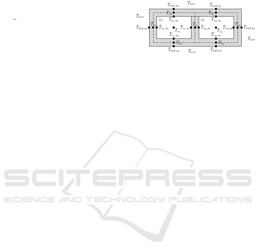
Figure 1: Thermal modeling of a two-zone building.
As an example, the diagram in Fig. 1 represents all
the temperatures involved in the thermal modelling of
a two-zone building. This simplified sketch, which
shows a 2D horizontal cross-sectional view, assumes
zones with no ceiling and no floor. 23 temperature
nodes are useful for modeling this building: T
z
∈ R
2
,
T
z,s
∈ R
8
, T
Ext,s
∈ R
6
, T
s
∈ R
7
.
2.3 EMPC - Economic Cost Function
and Constraints
The principle of predictive control (Rockett and Hath-
way, 2017) is to optimize a cost function to describe
the control objectives over a forecast time horizon
N
P
. At each instant k, an optimal control sequence
{u
∗
(k + j))}
1≤ j≤N
P
is calculated to minimize this
function and only the first element u
∗
(k + 1) is ap-
plied to the system. The economic objective function
J
MPC
(u,x) that we propose in the context of the ther-
mal regulation of a multizone building is as follows:
J
MPC
(u,x) = min
u
N
P
∑
j=1

k
T
O p
(k + j) − T
C
(k + j)
k
2
Ψ
j
+
k
u(k + j)
k
2
e
u
j
+
k
∆u(k + j)
k
2
e
0
∆u
j

(7)
with:
• T
T
C
(k + j) =

T
C,z
1
(k + j) . . . T
C,z
N
(k + j)

∈ R
N
and T
T
O p
(k+j)=

T
O p,z
1
(k+j). . . T
O p,z
N
(k+ j)

∈ R
N
the estimated operative temperature in each zone
z
i
according to model (6);
•
k
T
O p
(k + j) − T
C
(k + j)
k
2
Ψ
j
=
N
∑
i=1
ψ
z
i
, j
|
T
O p,z
i
(k + j) − T
C,z
i
(k + j)
|
2
•
k
u(k + j)
k
2
e
u
j
=
N
∑
i=1
N
S
∑
ξ=1
e
ξ,z
i
, j


u
ξ,z
i
(k + j)


2
;
•
k
∆u(k + j)
k
2
e
0
∆u
j
=
N
∑
i=1
N
S
∑
ξ=1
e
0
ξ,z
i
, j


u
ξ,z
i
(k + j) − u
ξ,z
i
(k + j − 1)


2
-Regularized Economic Model Predictive Control for Thermal Comfort in Multizone Buildings
139

• According to models (5) and (6), all control inputs
can be grouped according to the vectors u
z
i
(k),
u(k + j) and u defined as follows:





u
T
z
i
(k) =

u
HP
z
i
(k) u
CMV
z
i
(k) u
TTW
z
i
(k) u
VB
z
i
(k)

u
T
(k + j)=

u
T
z
1
(k + j) . . . u
T
z
N
(k + j)

u
T
=

u
T
(k + 1) . . . u
T
(k + N
P
)

(8)
• Weightings e
ξ,z
i
, j
and e
0
ξ,z
i
, j
make it possible to
specify the cost in euros of each of the possible
actions on the system. The e-terms will reflect the
energy cost of starting a HP or a VMC for a period
of time while the e
0
-terms will reflect the opening
or closing of tilt-turn windows or venetian blinds.
As for ψ
z
i
, j
, it reflects the importance attached to
T
O p,z
i
(k + j) being close to T
C,z
i
(k + j).
Remark 1: The minimization of J
MPC
(u,x) (7)
requires the calculation of the operative temperature
T
O p
in each zone z
i
. According to the definition
(1), this calculation requires not only the knowledge
or estimation of the temperature of each surface in
contact with these zones, but also their prediction
over the forecast time horizon N
p
. In a properly
insulated building, since the ambient air temperature
in each zone z
i
is generally not very different from the
mean radiant temperature, it is common to consider
T
z
rather than T
O p
in the definition of criterion
J
MPC
(u,x).
In the long term, the economic cost of a control sce-
nario is not reduced to the mere expression of crite-
rion (7). Indeed, the latter does not take into account
abnormal wear and tear or premature failure of actu-
ators, which can generate significant additional costs.
In the building context, for example, it is recognized
that increasing the number of on/off cycles of a HP
compressor increases its electrical consumption but
also its wear and tear. Therefore, when synthesizing
the control scenario {u
∗
(k + j)}
1≤ j≤N
P
over a horizon
N
P
, it is important to reduce as much as possible this
number of on/off cycles for this equipment.
In order to minimize criterion J
MPC
(u,x) while
taking into account this last remark, a regularisation
term is added.
3 REGULARIZED EMPC
(REMPC)
3.1 Regularized Criterion
It is proposed to consider a regularized criterion such
as:
J
λ,Ω
(u) = (1 − λ)J
MPC
(u,x) +λΩ (u) (9)
with J
MPC
(u,x) defined by (7) and where 0 ≤ λ ≤ 1
is a regularization parameter. The additional term
λΩ(u) in the criterion amounts to regularizing the so-
lution through a penalty of the latter. In the context
of the problem presented before, λΩ (u) must be a
penalty that favours the parsimony of the first deriva-
tive of u. Based on Tikhonov’s regularization method
(Engl et al., 1996), one possible technique is to in-
clude a linear operator R in the regularization term
Ω(u), and solve the following problem :
u
∗
λ,p
=argmin
u∈R
n
u
(1−λ)J
MPC
(u,x)+λ
k
Ru
k
min(1,p)
p
(10)
where k · k
p
is the `
p
-norm
k
w
i
k
p
:
=
n
w
i
∑
i=1
|
w
i
|
p
!
1
p
for a vector w
i
∈ R
n
w
i
. The power min(1, p) of the
regularization term
k
Ru
k
min(1,p)
p
makes it possible to
consider by continuity the `
∞
-norm of Ru for p → ∞:
lim
p→∞
k
Ru
k
min(1,p)
p
= lim
p→∞
∑
i
|
(Ru)
i
|
p
!
1
p
=
k
Ru
k
∞
(11)
and the `
0
-norm of Ru for p → 0:
lim
p→0
k
Ru
k
min(1,p)
p
= lim
p→0
∑
i
|
(Ru)
i
|
p
!
=
k
Ru
k
0
(12)
Equation (12) is particularly interesting because, from
a theoretical point of view, the parsimony of Ru is
measured using its `
0
-norm corresponding to the total
number of non-zero elements:
k
Ru
k
0
= #(i|(Ru)
i
6= 0) (13)
The linear transform R can take different forms:
• 0
th
-order regularization favouring solutions with a
small norm:
R = R
0
= I (14)
• 1
st
-order regularization. It consists in focusing a
priori on the low oscillating nature of the solution,
and thus penalizing rapid variations:
R = R
1
=








−1 1 0 0
0
0
0 0 −1 1








(15)
We notice that at 0
th
-order, the product Ru represents
a discretization of the vector u, while at 1
st
-order it is
a discretization of its first derivative.
SMARTGREENS 2020 - 9th International Conference on Smart Cities and Green ICT Systems
140

3.2 `
p
Penalization
There are several types of penalty functions (Hastie
et al., 2009). The Ridge regression corresponds to
a penalty of type `
2
-norm. As we will see below
through a simple example, this function has the par-
ticularity of not cancelling the coefficients of Ru but
rather reducing them and making them tend towards
0. This is a “shrinkage” of coefficients. The Lasso re-
gression, introduced by Tibshirani (Tibshirani, 1994),
is a regression penalized by the `
1
-norm of the coeffi-
cients of Ru, which favours parsimony. Fused-Lasso
is a variant which allows to take into account the spa-
tiality of the variables (Tibshirani et al., 2005). The
objective is to have close estimates for the same vari-
able when they are ”close in time”. This is made pos-
sible by penalizing the `
1
-norm of the difference of
this variable in two successive instants.
An even more natural penalization than
k
Ru
k
1
is to consider a constraint
k
Ru
k
ε
ε
(with 0 ≤ ε  1),
which not only contracts the value of the different el-
ements of Ru but also forces certain elements u
i
to be
strictly zero for λ large enough thanks to the shape of
the isolines of
k
Ru
k
ε
ε
.
By way of illustration, we consider the criterion:
J
λ,p
(u) = (1 − λ)J
1
(u) + λ
k
Ru
k
min(1,p)
p
(16)
with R = I (14) and J
1
(u) = (u
1
− 2 + u
2
)
2
+
(u
2
− 0.5)
2
.
First, we observe that ∀p ≥ 0, we have:



u
∗
0,p
=

1.5 0.5

T
= argmin
u
J
1
(u)
u
∗
∞,p
=

0 0

T
= argmin
u
k
Ru
k
min(1,p)
p
Between these two extreme values, the trajectory of
Γ
λ,p
followed by the minimum u
∗
λ,p
of J
λ,p
(u) as a
function of λ is represented in the u
1
−u
2
plane in red
in Fig. 2. The ellipsoids and the filled contour plot in
the background of these figures are isolines of J
1
(u)
and
k
Ru
k
min(1,p)
p
respectively. We can see on each of
the subfigures (Fig. 2a-2d) that the shape of the trajec-
tories Γ
λ,p
is very different according to the values of
p.
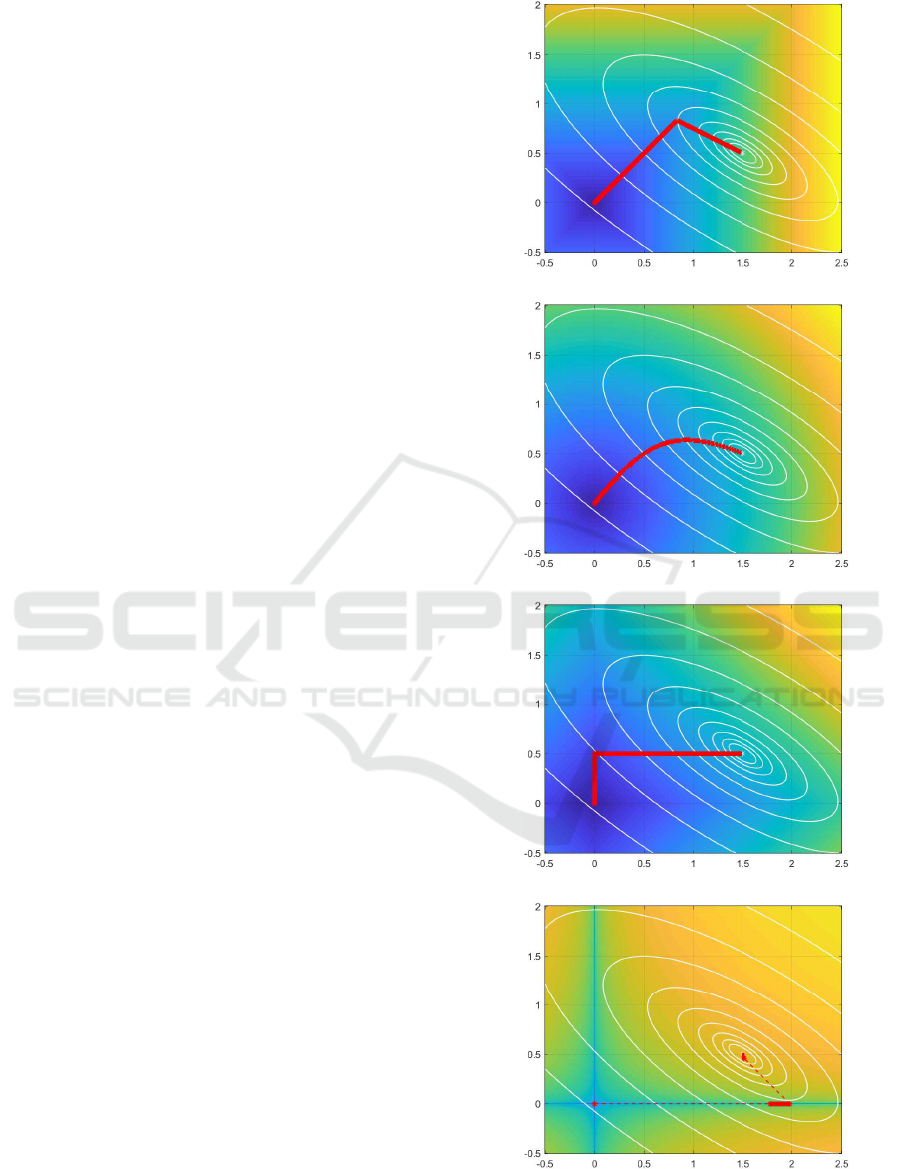
In particular, the LASSO selection (Fig. 2c) re-
sults in a more parsimonious solution than the Ridge
selection (Fig. 2b), which tends to make the coeffi-
cients very small without cancelling them. More gen-
erally, for p > 1, the trajectory Γ
λ,p
tends towards
u
∗
∞,p
for λ increasing but without being “attracted” by
the axes u
1
= 0 and u
2
= 0. On the other hand, as
soon as p ≤ 1, we observe that this convergence to-
wards u
∗
∞,p
takes place along one of the axes u
1
= 0
or u
2
= 0.
(a) p −→ ∞.
(b) p = 2.
(c) p = 1.
(d) p = 0.2.
Figure 2: Trajectory Γ
λ,p
(in red) followed by u
∗
λ,p
as a
fonction of λ in the u
1
− u
2
plane.
-Regularized Economic Model Predictive Control for Thermal Comfort in Multizone Buildings
141

In this context (p ≤ 1), it is interesting to point out
the difference in result between a regularization term
in `
ε
-norm and in `
1
-norm. It appears through this
example that the axis of attraction can be different
(u
2
= 0 for `
1
-norm (fig. 3c) vs. u
1
= 0 for `
0.2
-norm
(fig. 3d)). Given the shape of the isolines of J
1
(u),
the preferred solution (in the sense of minimizing the
criterion J
1
(u)) is the one associated with the lowest
p-value. Another phenomenon appears for p < 1; the
trajectory Γ
λ,p
followed by u
∗
λ,p
becomes discontin-
uous as the value of p decreases. This is due to the
non-convexity of the term
k
Ru
k
p
p
which increases
for small values of p and makes the criterion J
λ,p
(u)
non-convex.
4 APPLICATION TO THERMAL
COMFORT IN MULTIZONE
BUILDINGS
4.1 Regularized Criterion
With regards to the regularization term Ω(u), the fol-
lowing specifications are formulated:
• the number of on/off cycles for HP and CMV in
all zones z
i
should be limited. In view of the
previous paragraph, the minimisation of norms
N
∑
i=1


R
1
u
HP
z
i


ε
ε
and
N
∑
i=1


R
1
u
CMV
z
i


ε
ε
reflects this dual
objective with:
(
u
HP
z
i
=

u
HP
z
i
(k) | ˆu
HP
z
i
(k + 1) . . . ˆu
HP
z
i
(k + N
P
)

T
u
CMV
z
i
=

u
CMV
z
i
(k)| ˆu
CMV
z
i
(k+1). . . ˆu
CMV
z
i
(k+N
P
)

T
• the number of effective actuators should be lim-
ited at each time of prediction k + j and in each
zone z
i
. This specification translates as minimiz-
ing the term
N
∑
i=1


R
0
u
z
i
(k + j)


ε
ε
with u
z
i
(k + j)
the control vector defined by (8);
• the control inputs take values in the discrete set
{
0,1
}
(on/off or open/closed). The minimization
of the norm
k
R
0
(u  (u − 1))
k
ε
ε
meets this objec-
tive by defining by u  (u − 1) the element-wise
product of two vectors u and (u − 1).
For illustration purposes, the trajectory of Γ
λ,p
followed by the minimum u
∗
λ,p
of J
λ,p
(u) = (1 −
λ)J
1
(u) + λ
k
(u  (u − 1))
k
min(1,p)
p
as a function
of λ is represented in the u
1
− u
2
plane in red in
Fig. 3. For this example, we observe that Γ
λ,p
tends towards

1 1

T
=

on on

T
, which is the
on/off control associated with the lowest value of
J
1
(u). For this type of regularization, the choice
of a `
ε
-norm is also justified because the appear-
ance of the isolines J
1
(u) is not modified by con-
sidering J
λ,0
(u) knowing that
k
u  (u − 1)
k
0
=
dim(u) = 2 for all u except for axes u
1
= 0 and
u
2
= 0. This property is interesting because the
sole purpose of this regularization term is to im-
pose discrete values on u and not to modify the
shape of the isolines;
Therefore, Ω(u) is defined as:
Ω(u) = α
1





R
0
NB
K
i=1
(u − u
i
1)
!





ε
ε
+
N
∑
i=1

α
2


R
1
u
HP
z
i


ε
ε
+ α
3


R
1
u
CMV
z
i


ε
ε

+α
4
N
∑
i=1
N
P
∑
j=1


R
0
u
z
i
(k + j)


ε
ε
(17)
with:
• u and u
z
i
(k + j): augmented control vectors (8);
•
NB
K
i=1
(u − u
i
1) = (u −u
1
1)  . . .  (u − u
NB
1)
where  is the element-wise product of two
vectors and (u
i
)
1≤i≤NB
represent some constant
values that can be taken by at least one of the
control inputs. For on/off controls, we have
NB = 2, u
1
= 1 (on) and u
2
= 0 (off);
• u
TTW
z
i
=

u
TTW
z
i
(k) | ˆu
TTW
z
i
(k+1) .. . ˆu
TTW
z
i
(k+N
P
)

T
;
• u
VB
z
i
=

u
VB
z
i
(k) | ˆu
VB
z
i
(k+1) . . . ˆu
VB
z
i
(k+N
P
)

T
.
An α
2
(or α
3
) that tends towards 0 will generally
cause permanent stress on the associated actuator,
which will affect its lifetime. Conversely, an α
2
(or
α
3
) that tends towards infinity ensures a low stress
on the actuator but thermal comfort performance can
them become poor according to criterion J
MPC
(u,x)
because the solution obtained then becomes too far
from the optimal non-regularized solution.
4.2 Minimisation of the Regularized
Criterion
The closed-loop REMPC requires an optimal solu-
tion to (9) at each step. It is usually very difficult
to quickly find optimal solutions (and prove their op-
timality) for non-convex problems. First of all, it
is important to mention that the minimization of the
SMARTGREENS 2020 - 9th International Conference on Smart Cities and Green ICT Systems
142

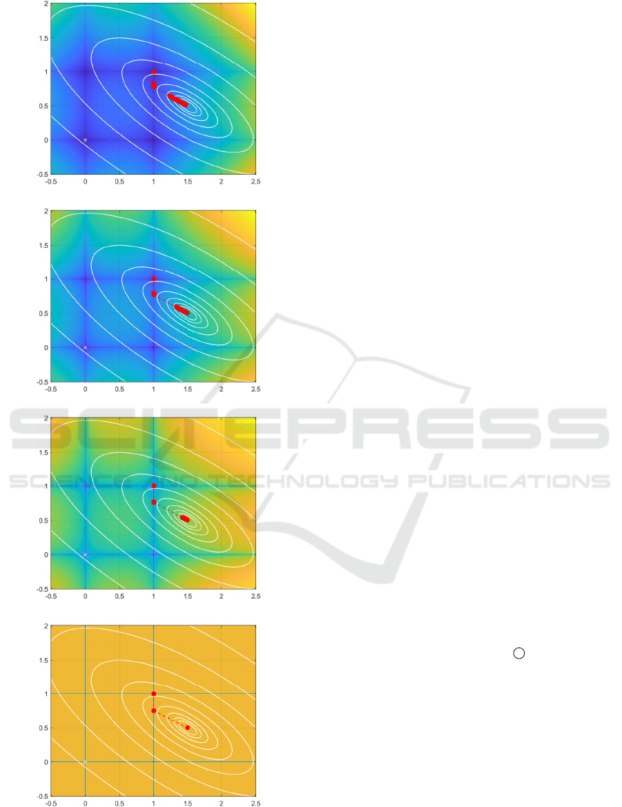
(a) p = 0.6.
(b) p = 0.4.
(c) p = 0.2.
(d) p = 0.
Figure 3: Trajectory Γ
λ,p
(in red) followed by u
∗
λ,p
as a
fonction of λ in the u
1
− u
2
plane.
non-regularized economic cost function J
MPC
(u,x)
constrained by the time-varying model (6) does not
present an analytical solution mainly because of the
input matrix B
ξ

x
z
(k), q
Sol
z
(k), T
Ext
(k)

, which de-
pends on the chosen control scenario. Thus, even
if the non-convexity of the `
ε
-norm makes NP-Hard
the regularized optimization problem, the complexity
of the solving algorithm is not significantly increased
with the regularization term. Although solvers such
as “Interior Point OPTimizer” (IPOPT) (W
¨
achter and
Biegler, 2006) can efficiently find local solutions to
nonlinear programming problems, these solutions are
not particularly suited to our problem.
To solve this problem, we use a recently devel-
oped iterative algorithm (Gabsi et al., 2018b), the ob-
jective of which is to estimate the optimal control sce-
nario with a controlled computation load. The idea is
to keep at each time of prediction k + j only a limited
number of scenarios among all those that are possi-
ble. For this purpose, main component analysis is
performed on a limited number of points judiciously
chosen in the variables space (T
O p,z
1
(k + j),T
O p,z
2
(k +
j), . . . , T
O p,z
N
(k + j)) in order to determine a suitable
basis for the representation of all possible realizations
of T
O p,z
i
(k + j) with i = 1, . . . , N. By prioritizing the
information, this makes it possible to replace the set
of all these realizations by a smaller subset S
j
whose
cardinality is set a priori. This procedure is repeated
N
p
times in an iterative manner for j ranging from 1
to N
p
. Of course, the larger the number |S
j
|, the bet-
ter the approximation of the optimal control scenario.
This prioritization technique allows to consider not
only a non-convex regularized criterion J
λ,Ω
(u) (9)
but also important values for the forecast time hori-
zon N
P
.
4.3 Application to the “Eco-Safe”
Platform
The “Eco-Safe” platform consists of six zones and a
corridor (Fig. 4). Each zone z
i
= i is equipped with
several actuators and sensors to ensure a certain level
of thermal comfort. The “research and development”
room (R&D, zone z
1
) and the “handling” room (zone
z
5
) are frequently occupied by students. They have
a respective surface area of 51 m
2
and 34 m
2
. Four
other rooms, of 17 m
2
each, are used for the storage of
different materials. The temperature of zones z
1
and
z
5
can be controlled by two reversible air-to-air HPs
that can generate hot and cold air. A CMV also allows
air exchange between these two zones. A weather
station integrating several sensors communicates with
the platform and allows to know the different charac-
teristics of the outside air.
-Regularized Economic Model Predictive Control for Thermal Comfort in Multizone Buildings
143

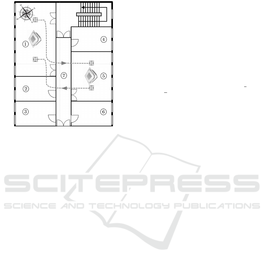
Figure 4: The “Eco-Safe” platform.
To illustrate the predictive control strategy presented
above, we used a dynamic model of this platform es-
tablished in (Gabsi et al., 2017). The latter integrates
the thermal behaviour of all partitions/walls/windows
in the zones as well as the different energy sources
(solar radiation, occupants in the premises, HPs). It is
possible to define 9 control scenarios:
• Scenario 0: no action on the system;
• Scenario 1: the CMV is switched on to circulate
air from zone z
5
to zone z
1
;
• Scenario 2: the CMV is switched on to circulate
air from zone z
1
to zone z
5
;
• Scenario 3: a HP is switched on in cooling mode
(constant air flow, outlet temperature equal to
291 K) in zone z
1
;
• Scenario 4: a HP is switched on in cooling mode
in zone z
5
;
• Scenario 5: both HPs are switched on in cooling
mode in zones z
1
and z
5
.
• Scenario 6: a HP is switched on in heating mode
(constant air flow, outlet temperature equal to
313 K) in zone z
1
;
• Scenario 7: a HP is switched on in heating mode
in zone z
5
;
• Scenario 8: both HPs are switched on in heating
mode in zones z
1
and z
5
.
The state-space model (6) associated with the plat-
form is:









x
z
(k + 1)=A
z
x
z
(k) + F
T
T
Ext
(k) + F
q
q
z
(k)+
8
∑
ξ=0
B
ξ
(x
z
(k), T
Ext
(k)) u
ξ
(k)
T
z
(k) = Cx
z
(k)
(18)
with:
• T
z
(k) =

T
z
1
, T
z
2
, T
z
4
, T
z
5
, T
z
7

T
(k); no surface
temperature is measured in zones z
i
;
• u(k)=

u
ξ
(k)

0≤ξ≤8
: the control vector formed of
0 and 1. It is defined as u
ξ
(k) = 1 and u
ξ
(k) = 0
for all ξ 6= ξ when scenario u
ξ
is implemented at
time k;
• q
z
(k) =

T
Ext
, Occ, Sol
West
, Sol
East
, T
HP

T
(k);
• T
Ext
(k): the outside temperature;
• Occ(k): the number of occupants in zone z
1
;
• Sol
West
(k) and Sol
East
(k): the energy provided by
solar radiation for zones z
1
, z
2
, z
3
and z
4
, z
5
, z
6
resp.;
• T
HP
(k): the temperature of the air forced through
the HPs, T
HP
(k) = 291 K (cooling mode) or 313 K
(heating mode).
Since the size of state vector x
z
is very large (72-
dimensional), the calculations required to develop a
predictive control would become very complicated
and time-consuming. The definition of a reduced or-
der model is therefore necessary, based on a balanced
state-space realization. In addition, as the purpose
of this application example is mainly to demonstrate
the interest of the regularisation terms, for the sake
of simplicity and in accordance with Remark 1, the
ambient air temperature in each zone z
i
is considered
into the economic cost function J
MPC
(u,x) (7), instead
of the operative temperature:
J
MPC
(u,x)=min
u
N
P
=12
∑
j=1
k
T
z
(k+j)−293
k
2
Ψ
j
+
k
u(k+j)
k
2
e
u
j
(19)
The reduced state vector is defined to correspond to
the ambient air temperatures measured in each zone
z
1
, z
2
, z
4
, z
5
and z
7
. Horizon N
p
is chosen equal to 12
due to the sampling period which is 5mn. The fore-
cast time horizon is therefore one hour depending on
the platform’s heating and cooling capacities. The
weighting matrix Ψ
j
is diagonal and time-variant.
The ith term of diagonal (Ψ
j
)
i,i
is zero if zone z
i
is
unoccupied at the time of prediction k + j. Otherwise,
this term, which is chosen equal to ψ
z
i
> 0, makes it
possible to give more or less importance to the en-
ergy criterion (second part of (19)) compared to the
SMARTGREENS 2020 - 9th International Conference on Smart Cities and Green ICT Systems
144

performance criterion (first part of (19)). For this il-
lustration example, we will assume that only zone z
1
is occupied during standard working hours. The term
k
∆u(k + j)
k
2
e
0
∆u
j
is not taken into account in the rela-
tionship (19) because the platform does not have au-
tomated closing/opening of tilt and turn windows or
venetian blinds. As for the diagonal matrix e
u
j
, it is
defined according to the energy consumption of each
of the scenarios (which is assumed to be constant no
matter the day and time), namely:
e
u
j
=
1
12
×diag

0 30 30 10
3
10
3
2000 10
3
10
3
2000

The regularisation term Ω(u) (17) takes the following
form:
Ω(u)=α
1
kR
0
u(u−1)k
ε
ε
+α
2



R
1
u
HP
z
1


ε
ε
+


R
1
u
HP
z
5


ε
ε

+α
2



R
1
u
CMV
z
1


ε
ε
+


R
1
u
CMV
z
5


ε
ε

(20)
with a very large value for α
1
. Regularization param-
eter λ (9) is taken as 0.5.
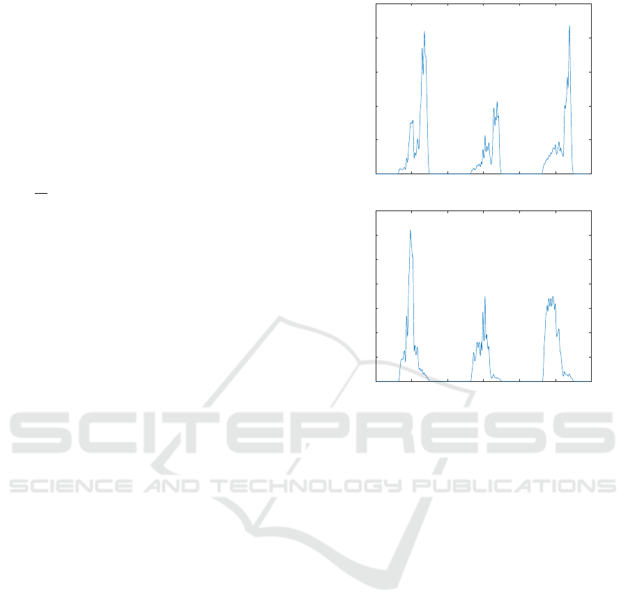
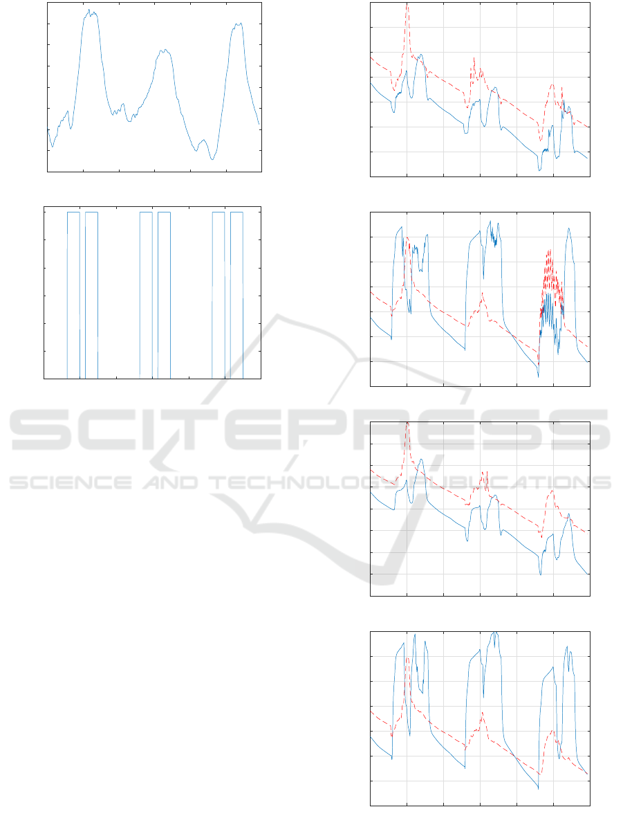
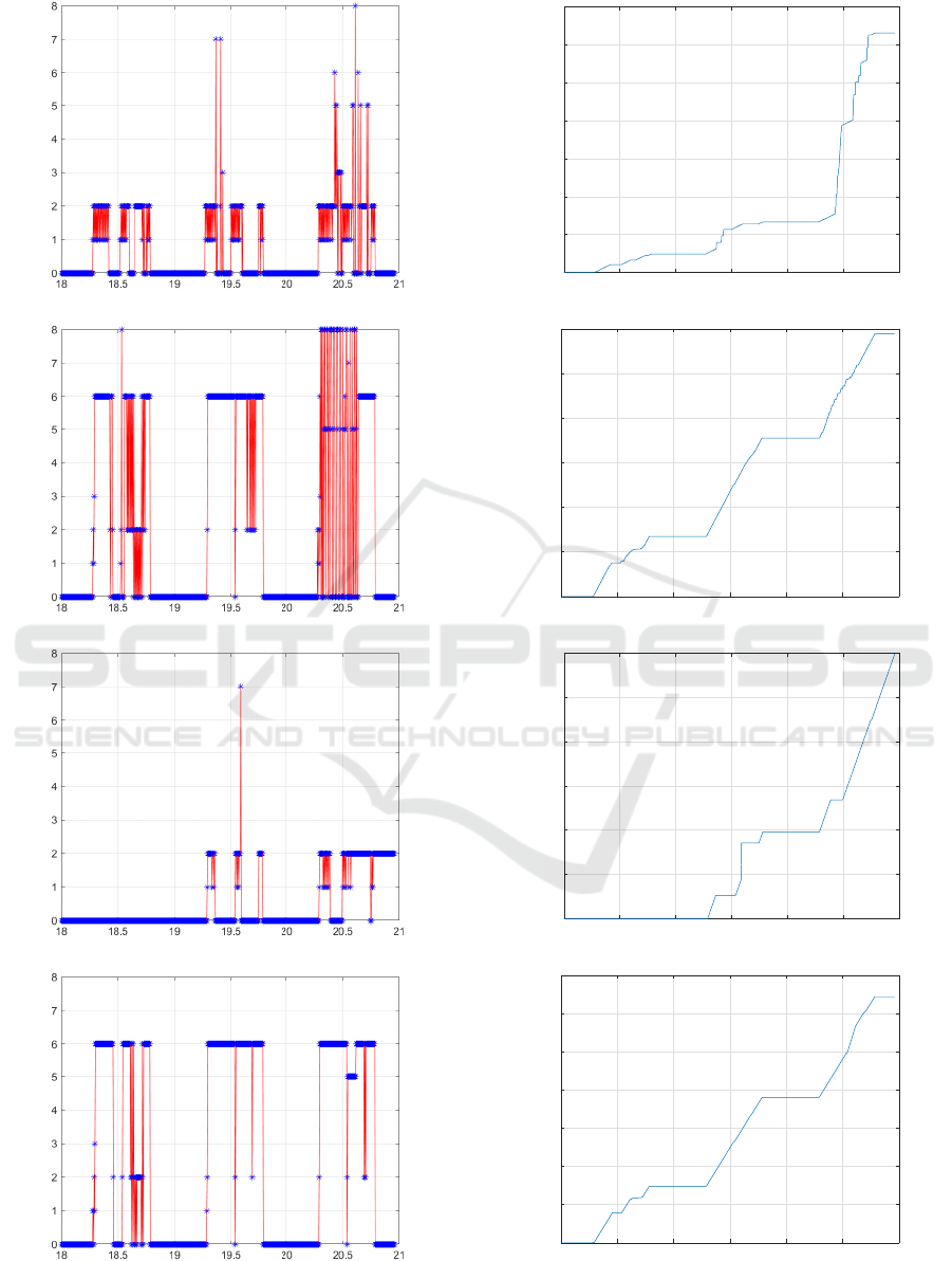
Fig. 7a to 7d represent over the period from 18
to 20 February 2019 the evolution of the ambient air
temperatures T
z
1
(k) and T
z
5
(k) respectively associated
with the control scenarios in Fig. 8a to 8d. The cumu-
lative energy cost (in kWh) for each of these scenarios
is shown in Fig. 9a to 9d respectively. The weather
conditions present during this period at the platform
location (Nancy, France) are reflected in Fig. 5a, 5b
and 6a. The first two show the daily evolution of the
solar energy entering the platform zones according to
their orientation. The third figure shows the evolu-
tion of the outside temperature in K. Fig. 6b finally
shows the number of occupants in zone z
1
(we will
assume that each person emits 80W of internal heat
gain). Fig. 8 represents as a function of time the value
of the index ξ associated with the non-zero element
of the vector u(k). A blue cross on a line ξ of these
figures at time k therefore reflects the implementation
of scenario ξ on the platform (u
ξ
(k) = 1). For exam-
ple, Fig. 8c shows that the non-zero element of u(k)
over the entire first day is u
0
(k). This control scenario
is associated with parameters ψ
z
1
= 1 and α
2
= 3. A
simple analysis of these different figures shows:
• the influence of parameter ψ
z
1
. The larger this
parameter is compared to the terms of e
u
j
, the
greater the proportion of criterion J
MPC
(u,x) re-
lated to comfort performance increases at the ex-
pense of energy consumption. However, the lower
this parameter is, the more important the energy
aspect becomes compared to thermal comfort.
• the interest of the regularization term related to
α
2
. By comparing Fig. 8a and 8b with Fig. 8c
18 18.5 19 19.5 20 20.5 21
0
50
100
150
200
250
(a) Sol
West
(k); z
i
= z
1
,z
2
,z
3
.
18 18.5 19 19.5 20 20.5 21
0
100
200
300
400
500
600
700
(b) Sol
East
(k); z
i
= z
4
,z
5
,z
6
.
Figure 5: Energy (W/m
2
) provided by solar radiation for
zones z
i
.
and 8d respectively, it is clear that an increase in
α
2
significantly reduces the number of switching
(on/off) of VMCs and HPs. A direct consequence
is the almost complete disappearance of the oscil-
lations observed on T
z
1
(k) and T
z
5
(k) (Fig. 7d vs.
Fig. 7b).
• the interest of the regularization term in α
1
which
allows to privilege discontinuous optimal values
for u during the optimization of the regularized
criterion. For this illustration example, only val-
ues 0 and 1 are allowed for all elements of u.
5 CONCLUSION
This paper aims to optimize the energy efficiency
of multizone buildings by implementing a regular-
ized economic model predictive controller (REMPC).
More precisely, the objective is to maintain thermal
comfort in occupied zones while minimizing energy
consumption.
To achieve this long-term overall objective, an
economic cost function was first defined and control
specifications were added via a regularization crite-
-Regularized Economic Model Predictive Control for Thermal Comfort in Multizone Buildings
145

18 18.5 19 19.5 20 20.5 21
272
274
276
278
280
282
284
286
288
(a) Outside temperature T
Ext
(K).
18 18.5 19 19.5 20 20.5 21
0
5
10
15
20
25
30
(b) Number of occupants Occ.
Figure 6: Disturbances q(k) (in addition to solar radiation).
rion. The first regularized term concerns the limita-
tion of the frequency of on/off cycles for particular
actuators such as HPs or VMCs. Indeed, the very fre-
quent starting and stopping of this type of equipment
makes inefficient their energy operating mode and can
especially lead to severe damages. Other criteria re-
lated to the number of actuators used at a given time
or to the discrete nature of certain control variables
were also taken into account in the regularized crite-
rion. An analysis showed the importance of choosing
an appropriate `
p
-norm to define these regularization
terms. It has been shown that a `
ε
-norm is to be pre-
ferred.
This control strategy was tested on a platform sim-
ulator (Gabsi et al., 2017) located in the CRAN labo-
ratory (Nancy/France) and gave very encouraging re-
sults for on-site implementation.
ACKNOWLEDGEMENTS
This work has financial support from the Contrat
de Plan Etat-R
´
egion (CPER) 2015-2020, project
”Mat
´
eriaux, Energie, Proc
´
ed
´
es”.
18 18.5 19 19.5 20 20.5 21
287
288
289
290
291
292
293
294
(a) ψ
z
1
= 1, α
2
= 0.
18 18.5 19 19.5 20 20.5 21
288
289
290
291
292
293
294
295
(b) ψ
z
1
= 20, α
2
= 0.
18 18.5 19 19.5 20 20.5 21
286
287
288
289
290
291
292
293
294
(c) ψ
z
1
= 1, α
2
= 3.
18 18.5 19 19.5 20 20.5 21
288
289
290
291
292
293
294
295
(d) ψ
z
1
= 20, α
2
= 10.
Figure 7: Ambient air temperatures T
z
1
(K, in solid blue
line) and T
z
5
(K, in red dashed line).
SMARTGREENS 2020 - 9th International Conference on Smart Cities and Green ICT Systems
146

(a) ψ
z
1
= 1, α
2
= 0.
(b) ψ
z
1
= 20, α
2
= 0.
(c) ψ
z
1
= 1, α
2
= 3.
(d) ψ
z
1
= 20, α
2
= 10.
Figure 8: Control scenarios.
18 18.5 19 19.5 20 20.5 21
0
0.5
1
1.5
2
2.5
3
3.5
(a) ψ
z
1
= 1, α
2
= 0.
18 18.5 19 19.5 20 20.5 21
0
5
10
15
20
25
30
(b) ψ
z
1
= 20, α
2
= 0.
18 18.5 19 19.5 20 20.5 21
0
0.1
0.2
0.3
0.4
0.5
0.6
(c) ψ
z
1
= 1, α
2
= 3.
18 18.5 19 19.5 20 20.5 21
0
5
10
15
20
25
30
35
(d) ψ
z
1
= 20, α
2
= 10.
Figure 9: Cumulative energy cost (kWh).
-Regularized Economic Model Predictive Control for Thermal Comfort in Multizone Buildings
147

REFERENCES
Aguilera, R. P., Delgado, R., Dolz, D., and Ag
¨
uero, J. C.
(2014). Quadratic MPC with l
0
-input constraint. IFAC
Proceedings Volumes, 47(3):10888 – 10893.
Aguilera, R. P., Urrutia, G., Delgado, R. A., Dolz,
D., and Ag
¨
uero, J. C. (2017). Quadratic model
predictive control including input cardinality con-
straints. IEEE Transactions on Automatic Control,
62(6):3068–3075.
Amy, T., Kong, H., Auger, D., Offer, G., and Longo, S.
(2016). Regularized MPC for power management of
hybrid energy storage systems with applications in
electric vehicles. IFAC-PapersOnLine, 49(11):265 –
270.
Challapalli, N., Nagahara, M., and Vidyasagar, M. (2017).
Continuous hands-off control by clot norm minimiza-
tion. IFAC-PapersOnLine, 50(1):14454 – 14459. 20th
IFAC World Congress.
Cho, K.-j. and Cho, D.-w. (2018). Solar heat gain coeffi-
cient analysis of a slim-type double skin window sys-
tem: Using an experimental and a simulation method.
Energies, 11(1).
Cojocaru, E. G., Bravo, J. M., Vasallo, M. J., and Mar
´
ın, D.
(2020). A binary-regularization-based model predic-
tive control applied to generation scheduling in con-
centrating solar power plants. Optimal Control Appli-
cations and Methods, 41(1):215–238.
Ellis, M., Durand, H., and Christofides, P. D. (2014). A
tutorial review of economic model predictive control
methods. Journal of Process Control, 24(8):1156 –
1178.
Engl, H. W., Hanke, M., and Neubauer, A. (1996). Regu-
larization of inverse problems, volume 375. Springer
Science & Business Media.
Gabsi, F., Hamelin, F., Pannequin, R., and Chaabane, M.
(2017). Energy efficiency of a multizone office build-
ing: MPC-based control and simscape modelling. In
2017 International Conference on Smart Cities and
Green ICT Systems (SMARTGREENS), pages 227–
234, Porto, Portugal. INSTICC.
Gabsi, F., Hamelin, F., and Sauer, N. (2018a). Building hy-
grothermal modeling by nodal method. In 2018 IEEE
PES Innovative Smart Grid Technologies Conference
Asia (ISGT), Singapore.
Gabsi, F., Hamelin, F., and Sauer, N. (2018b). Hygrother-
mal modelling and MPC-based control for energy and
comfort management in buildings. In 2018 Interna-
tional Conference on Smart Grid and Clean Energy
Technologies (ICSGCE), Kajang, Malaysia.
Gallieri, M. and Maciejowski, J. M. (2012). l
asso
MPC:
Smart regulation of over-actuated systems. In 2012
American Control Conference (ACC), pages 1217–
1222.
Gallieri, M. and Maciejowski, J. M. (2015). Model predic-
tive control with prioritised actuators. In 2015 Euro-
pean Control Conference (ECC), pages 533–538.
Godina, R., Rodrigues, E. M. G., Pouresmaeil, E., Matias,
J. C. O., and Catal
˜
ao, J. P. S. (2018). Model predic-
tive control home energy management and optimiza-
tion strategy with demand response. Applied Sciences,
8(3).
Hastie, T., Tibshirani, R., and Friedman, J. (2009). The el-
ements of statistical learning: data mining, inference
and prediction. Springer, 2 edition.
McCartney, K. J. and Nicol, J. F. (2002). Developing an
adaptive control algorithm for europe. Energy and
Buildings, 34(6):623 – 635. Special Issue on Thermal
Comfort Standards.
Nagahara, M., Quevedo, D. E., and Østergaard, J. (2014).
Sparse packetized predictive control for networked
control over erasure channels. IEEE Transactions on
Automatic Control, 59(7):1899–1905.
Pakazad, S. K., Ohlsson, H., and Ljung, L. (2013). Sparse
control using sum-of-norms regularized model predic-
tive control. In 52nd IEEE Conference on Decision
and Control, pages 5758–5763.
Rao, C. V. (2018). Sparsity of linear discrete-time optimal
control problems with l
1
objectives. IEEE Transac-
tions on Automatic Control, 63(2):513–517.
Rawlings, J. B., Patel, N. R., Risbeck, M. J., Maravelias,
C. T., Wenzel, M. J., and Turney, R. D. (2018). Eco-
nomic MPC and real-time decision making with ap-
plication to large-scale HVAC energy systems. Com-
puters & Chemical Engineering, 114:89 – 98.
Rockett, P. and Hathway, E. A. (2017). Model-predictive
control for non-domestic buildings: a critical review
and prospects. Building Research & Information,
45(5):556–571.
Serale, G., Fiorentini, M., Capozzoli, A., Bernardini, D.,
and Bemporad, A. (2018). Model predictive con-
trol (MPC) for enhancing building and HVAC system
energy efficiency: Problem formulation, applications
and opportunities. Energies, 11(3).
Tibshirani, R. (1994). Regression shrinkage and selection
via the lasso. Journal of the Royal Statistical Society,
Series B, 58:267–288.
Tibshirani, R., Saunders, M., Rosset, S., Zhu, J., and
Knight, K. (2005). Sparsity and smoothness via the
fused lasso. Journal of the Royal Statistical Society.
Series B (Statistical Methodology), 67(1):91–108.
W
¨
achter, A. and Biegler, L. (2006). On the implemen-
tation of an interior-point filter line-search algorithm
for large-scale nonlinear programming. Mathematical
programming, 106:25–57.
Zhuang, J., Chen, Y., and Chen, X. (2018). A new simpli-
fied modeling method for model predictive control in
a medium-sized commercial building: A case study.
Building and Environment, 127:1 – 12.
Zong, Y., B
¨
oning, G. M., Santos, R. M., You, S., Hu, J.,
and Han, X. (2017). Challenges of implementing eco-
nomic model predictive control strategy for buildings
interacting with smart energy systems. Applied Ther-
mal Engineering, 114:1476 – 1486.
SMARTGREENS 2020 - 9th International Conference on Smart Cities and Green ICT Systems
148