An FCA-based Approach to Direct Edges in a Causal Bayesian Network:
A Pilot Study using a Surgery Data Set
Walisson Ferreira
1
, Mark Song
2
and Luis Zarate
2
1
Centro Universit
´
ario UNA, Brazil
2
Pontificia Universidade Cat
´
olica de Minas Gerais, Brazil
Keywords:
Causal Inference, Formal Concept Analysis, FCA, Markov Equivalence, Causal Bayesian Networks, Causal
Relationship, Bayesian Networks, Attributes Implication.
Abstract:
One of the problems during the construction of Causal Bayesian Network based on constraint algorithms
occurs when it is not possible to orient edges between nodes due to Markov Equivalence. In this scenario this
article presents the use of Formal Concept Analysis (FCA), specially attributes implication, as an alternative
to support the definition of the direction of the edges. To do this it was applied algorithms of Bayesian
learners (PC) and FCA in a data set containing 12 attributes and 5,473 records of surgeries performed in
Belo Horizonte - Brazil. According to the results, although attribute implication did not necessarily mean
causality, the implication rules were useful in defining edges orientation on the Bayesian network learned by
PC Algorithm. The results of FCA were validated through intervention using do-calculus and by an expert in
the domain. Therefore, as result of this paper, it is presented a heuristic to direct edges between nodes when
the direction is unknown.
1 INTRODUCTION
Since Judea Pearl conquered the Alan Turing prize in
2011 ”For fundamental contributions to artificial in-
telligence through the development of a calculus for
probabilistic and causal reasoning”, Causal Inference
is a research area that has been challenging many re-
searchers from different fields of knowledge.
A significant amount of research applying Causal
Inference had been developed over the last years. Re-
searches such as feature selection, (Guyon and Alif-
eris, 2007) and (Tsamardinos et al., 2019), missing
data, (Shpitser et al., 2015), discovery of knowledge
in many field such as education, (de Carvalho and
Zarate, 2019) and others.
One of the most common representation of the
causality relationship is Bayesian Network. In other
words, Bayesian Network theory has been used in or-
der to identify the causality relationship in a set of
observed variables.
Bayesian Network (BN) is a probabilistic graph-
ical model that represents a set of variables and its
probability distribution. It is represented by a Di-
rected Acyclic Graph (DAG) in which each edge rep-
resents a random variable and each arc linking two
nodes is interpreted as a direct influence from one
node to another.
A Causal Bayesian Network (CBN) is Bayesian
Network in which, in a DAG, the structure V
1
→ V
2
is
interpreted as a causal relationship, meaning that V
1
is a direct cause of V
2
. In other words, V
1
is the cause
and V
2
the effect of V
1
.
Constraint-based algorithms is one of most used
approach for learning Bayesian Network especially
those based on conditional independence. However,
these algorithms, such as PC (Spirtes et al., 2000),
which name stands for the initials of its inventors
Peter Spirtes and Clark Glymour, are not able to iden-
tify the true Bayesian Network due to the Observa-
tional Equivalence of Markov.
A set of Bayesian Network is Markov equiva-
lent, if the elements of the set represent the same
joint probability distribution. Therefore, Observa-
tional Equivalence is a limit for directing edges in
Bayesian Networks from probabilities, since, in most
cases, the algorithms determine the candidate’s causal
structures from the data set, not the true causal graph.
The state of art of constraint-based algorithms
(the approach used in this paper) is PC Algorithm
presented by (Spirtes et al., 2000). This algo-
rithm has as input a conditional probability table and
as output a set of DAG that are Markov equiva-
116
Ferreira, W., Song, M. and Zarate, L.
An FCA-based Approach to Direct Edges in a Causal Bayesian Network: A Pilot Study using a Surgery Data Set.
DOI: 10.5220/0009392101160123
In Proceedings of the 22nd International Conference on Enterprise Information Systems (ICEIS 2020) - Volume 1, pages 116-123
ISBN: 978-989-758-423-7
Copyright
c
 2020 by SCITEPRESS – Science and Technology Publications, Lda. All rights reserved

lent, known as Completed Partially Directed Acyclic
Graph (CPDAG). According to (Verma and Pearl,
1991), CPDAG is a good tool for representing equiv-
alent classes of Causal Model.
From CPDAG one can use background knowledge
to direct edges. The researcher can also make in-
terventions, using, for instance, do-calculus, (Pearl,
2009), to infer the causality relationship among vari-
ables when the graph is unknown (Hyttinen et al.,
2015).
Another area of study that has been used for data
analysis is Formal Concept Analysis (FCA). FCA is
a method proposed by Wille (Wille, 1982) in the
early 1980 and it is used for knowledge representation
through formal concepts that are hierarchically struc-
tured as lattice. Concept lattice and the knowledge
can also be represented using attribute implications.
So, FCA has two mayors’ outputs: i) concept lattice,
a ordered collection of formal concepts; ii) attribute
implications, the knowledge represented (
ˇ
Skopljanac
Ma
ˇ
cina and Bla
ˇ
skovi
´
c, 2014).
According to (Poelmans et al., 2013), FCA is the
main theme of more than 1,000 papers that have been
published in last years. In (Poelmans et al., 2013) the
authors stress that 20% of the articles on FCA is about
knowledge discovery.
Once that, in some scenarios, during the process
of generating the BN it is difficult to direct the edge,
it is necessary to find new approaches that make pos-
sible to identify which node, variable, is the cause and
which is the effect.
In this scenario, this article has as main objective
to present an approach based on the FCA, specially
implication rules, as a heuristic that tries to determine
a possible direction of the edge between two vertices
in a CPDAG when the identification is not possible
through conditional dependence. It is important to
stress that in our research we did not find another
work using FCA to direct edges in a Bayesian Net-
work, this means that it was not possible to compare
the results of this article with other.
The remainder of the paper is structured as follow.
Section 2 provides an overview of the main concepts
covered in the paper. In section 3, ours experiments
and results are presented. Finally, section 5, presents
some conclusions and future work.
2 THEORETICAL FOUNDATION
This section presents the main topics that support this
work: Causal Bayesian Networks and Formal Con-
cept Analysis.
2.1 Causal Bayesian Network
Formally, a Bayesian Network is pair B = (G,P), such
as G(V,E) represents the DAG and (P) the joint prob-
ability distribution over (V) that satisfies the Markov
condition. Markov condition states that each node
X ∈ V is independent of all of its non-descendant
nodes given its parents. In other words, each node
of G is conditionally independent of the set of all its
non-descendant nodes given its parents.
The definition of conditional independence states
that: given X,Y, Z ⊆ V , X and Y are conditionally
independent given Z, denoted X ⊥⊥ Y |Z, if and only if
P(X = x,Y = y|Z = z) = P(X = x|Z = z)P(Y = y|Z =
z) , for all values x, y, z of X, Y, Z respectively, such
that P(Z = z) > 0. The interpretation of conditional
independence is that learning about Y does not change
our knowledge about X, considering our beliefs in Z,
and vice versa.
Through graphs it is possible to observe the set of
variables that is relevant to each other. In a graph, the
independence relation among variable is represented
through the property called d-separation.
According to (Neapolitan, 2003), considering
G(V,E) a DAG, a set of vertices Z ⊆ V and X and
Y be distinct nodes, such that X,Y ⊆ V − Z, X and Y
are d-separated by Z in G, if every chain between X
and Y is blocked
1
by Z.
When a graph G represents the joint distribution
P, we say that G is an Independence map, I-map for
short, of P. In this case, X ⊥⊥
G
Y |Z ⇒ X ⊥⊥
P
Y |Z.
Fig. 1 shows an example of D-separation. The
Fig. 1 is a DAG with a chain from X
1
to X
3
that is
blocked by X
2
, so X
1
and X
3
are d-separated by X
2
.
Once that X
1
and X
3
are d-separated by X
2
, we can say
that X
1
is independent of X
3
given X
2
, X
1
⊥⊥ X
3
|X
2
.
Figure 1: Example of D-Separation.
Another advantage of using graph is the factorization
of the joint distribution. The chain rule states that giv-
ing a set of n events (E
1
, E
2
, ...E
n
) the probability of
join events can be written as a product of n conditional
probabilities, as follow:
P(E
1
, E
2
, ..., E
n
) =
P(E
n
|E
(
n − 1), ...E
2
, E
1
)...P(E
2
|E
1
)P(E
1
)
(1)
Thanks to Markov condition, Bayesian Networks rep-
resents the chain rule, equation 1, in a factorized way,
equation 2.
1
More details about d-separation can be found in section
11.1.2, d-Separation without Tears, (Pearl, 2009).
An FCA-based Approach to Direct Edges in a Causal Bayesian Network: A Pilot Study using a Surgery Data Set
117

P(X
1
, X
2
, ...X
n
) =
∏
j
P(x
j
|pa
j
) (2)
In equation 2, pa
j
is the Markovian Parents of x
j
. Ac-
cording to (Pearl, 2009), Markovian Parents is a min-
imal set of predecessors of x
j
that renders x
j
indepen-
dent of all its other predecessors.
Another assumption of constraint-based algo-
rithms is the Faithfulness Condition. G and P(V) sat-
isfy the Faithfulness Condition if and only if every
conditional independence relationship in P is repre-
sented in G. In other words, if there are two variables
that are probabilistically independent in P, there must
be an edge between them in G.
If P and G are faithful to each other, then G is a
perfect map, P-map for short, of P. On the other hand,
P is a DAG-Isomorph of G.
PC algorithm is the commonly method used to
learn Bayesian Network. The main idea behind
this algorithm is testing conditional independence be-
tween adjacent nodes given the other variables. PC
has as its input: vertex set, condition independence
information and significance level.
As presented in Table 1, PC algorithm is divided
in four stages. In the first step a complete undirected
graph is created. During the second stage, edges be-
tween the nodes, variables, are deleted based on the
conditional independence test. At the end of the sec-
ond stage of the algorithm is produced the skeleton,
the undirected version, of the graph G.
Table 1: PC Algorithm.
Input: Nodes,
Probabilistic distribution
hypothesis test (p-value)
Output: CPDAG
Stage 1: Construct the complete graph
Stage 2: Remove edges according to
condition independence information
Stage 3: Orient as v-structure
Stage 4: Orient as remaining edges
In the third step, triple of vertices X, Y, Z such that the
pairs X, Y and Y, Z are adjacents in G but the nodes
X and Z are not adjacents. These edges are oriented
according to the rules defined in (Spirtes et al., 2000).
This triple of edges is known as v-structures (Kalisch
et al., 2012) or immorality (Flesch and Lucas, 2007).
In the last step, the remaining edges are oriented
according to the rules defined in (Spirtes et al., 2000).
The output of PC algorithm is a CPDAG that rep-
resents the Markov equivalence class. Markov equiv-
alence occurs when two DAG have the same skeleton
and same set of v-structure (Flesch and Lucas, 2007).
Consider, for instance, the following conditional
independence: X
1
⊥⊥ X
3
|X
2
. From this distribution,
it is possible to identify three equivalents graphs as
shown in Fig. 2. Therefore, these three graphs com-
pound the Markov equivalence class.
Figure 2: Example of Markov Equivalence.
From the application of the PC algorithm in X
1
⊥⊥
X
3
|X
2
we obtain the CPDAG shown in Figure 3. The
CPDAG produced by PC has the same skeleton and
the same v-structure of every DAG in the equivalence
class, Figure 2.
Figure 3: Example of CPDAG.
In the CPDAG, edges that point in one direction are
those common to all DAGs in the equivalence class,
once that there is no common direct edge in the equiv-
alence class of Fig. 2, the resultant CPDAG, Fig. 3,
does not have directed edges.
According to (Pearl, 2009) bi-directed edges in a
CPDAG represent spurious relation. (Spirtes et al.,
2000) stress that a double-headed arrow may occurs
due to unmeasured common causes, in these case, the
assumption causal sufficiency would not be observed.
Therefore, besides Causal Markov Condition and
Faithfulness, PC algorithm also considers a third as-
sumption, Causal Sufficiency. This assumption states
that all common causes of the measured variables are
also measured. In other words, there are no hidden
confounders.
(Pearl, 2009) stress that links unidirectional in a
CPDAG denote genuine causation and those edges
that are undirected means that the relationship be-
tween the vertices remain undetermined.
In (Hyttinen et al., 2015) it is applied the so-called
do-calculus, developed by (Pearl, 2009), to identify
the true DAG. The main idea behind this theory is to
make interventions in the model to assure that there
is a causal relationship between attributes. The sim-
plest type of intervention is realized by inputting some
ICEIS 2020 - 22nd International Conference on Enterprise Information Systems
118

value, x
i
to variable, X
i
. This intervention is made
using do operator
2
: do(X
i
= x
i
) or by do(x
i
) (Pearl,
2009).
As a result of the interventions it is possible to
compute the Causal Effect of one variable in an-
other. Causal Effect of variable X on Y denoted by
P(Y |do(x)) is the marginal distribution of Y in the new
model under intervention.
Through interventions, it is possible to see, for
example, how the probability of Y would change if
X were observed P(Y |X), distinguishing it from the
probability of X being submitted to an experiment
P(Y |do(x)).
As pointed earlier in this paper, to orient an edge
in BN is a problem in which the solution it is limited
to background knowledge or intervention. So, this ar-
ticle will apply FCA, next section, to deal with this
issue.
2.2 Formal Concept Analysis
Formal Concept Analysis (FCA) is a mathematical
theory for knowledge representation, describing the
relationship, I, between a set of objects, G, and a set of
attributes, M. This relationship is called formal con-
text.
According to (Carpineto and Romano, 2004), for-
mal context is triple K := (G, M, I), such that I ⊆
G × M is an incidence relation of the context. To rep-
resent an element of I it is used (g, m) ∈ I or gIm, this
expression can be interpreted as an object g is in rela-
tion I with an attribute m. In other words, gIm means
that the object g has attribute m.
The cross-table shown in Table 2 is an example
of Formal Context. The meaning of each attribute is
detailed in table 3. In this example first.internment,
over.70.years, T.Ate.Maior.4, over.2.hour, Emergency,
ASA.2 are elements of the set M and P
1
, P
2
, P
3
, P
4
, P
5
and P
6
the set of objects, G. If an object has an at-
tribute a mark, X, is placed on the intersection of that
object’s row and that attribute’s column.
To extract formal concepts from formal context
it is used two operators called derivation operators.
Considering A ⊆ G and B ⊆ M, the derivation opera-
tors, (.)
0
, are:
• A
0
= {m ∈ M| gIm for all g ∈ A} ,
• B
0
= {g ∈ G| gIm for all m ∈ B} .
The first operator, A
0
, has as output the set of at-
tributes common to all the objects in A. The second
one, B
0
, the set of objects with all attributes in B.
2
Besides the do operator, do-calculus theory has a set of
rules that can be consulted in (Pearl, 2009).
Formal concept of the context (G,M,I) is pair of
sets (A,B) such that, given A ⊆ G and B ⊆ M, A
0
= B
and B
0
= A, A is called the extent and B the intent of
the formal concept (A,B).
For instance, from table 2, considering A =
{P
5
, P
6
} and B = {over.2.hour, Emergency} apply-
ing the second operator of derivation we have B
0
=
{P
1
, P
2
, P
3
, P
4
, P
5
, P
6
}. So, in this case A and B
is not a formal concept because B
0
6= A. On
the other hand, if we consider A = {P
2
, P
3
}, B =
{ f irst.internment, ASA.2, over.2.hour, Emergency},
then B
0
= {P
2
, P
3
} and A
0
= { f irst.internment,
ASA.2, over.2.hour, Emergency}. Once that A
0
= B
and B
0
= A, we have a formal concept.
Formal concepts can be expressed in terms of at-
tribute implication. Attribute implication is a pair of
set of attributes represented by A → B, where A, B ⊆
M. Formulas A → B have the following meaning:
each object having all attributes from A has also all
attributes from B.
Implications are also known as rules or if-then
statements. In the formula A → B, A is the premise
or antecedent and B the conclusion or consequent.
For a formal context K := (G, M, I) the implica-
tion A → B will hold, if and only if, A ⊆ B
00
is equiv-
alent to A
0
⊆ B
0
. (.)
00
is the double application of (.)
0
,
known as closure operator.
From table 2, for example, it is possible to extract
some rules of implication such as:
• T.over.4 over.2.hour Emergency → over.70.years
ASA.2;
• over.70.years over.2.hour Emergency → T.over.4
ASA.2
• first.internment over.2.hour Emergency → ASA.2
According to (Z
´
arate et al., 2008), the number of rules
that can be inferred from a formal context is exponen-
tial. Assuming that a data set can have n attributes,
there could be 2
2n
implications rules, many of them
are redundant or unnecessary.
In spite of not being a causal relationship, im-
plication rules such as P → Q means that P implies
Q. Therefore, there exist a temporal relationship that,
combined with other assumption, maybe a causality
relationship. This kind of relationship is one the keys
that motivate this study.
3 EXPERIMENTS AND RESULTS
As shown in Fig. 4, this work was developed using
two theories, Causal Inference and Formal Concept
Analysis. After applying Bayesian learner algorithm
An FCA-based Approach to Direct Edges in a Causal Bayesian Network: A Pilot Study using a Surgery Data Set
119

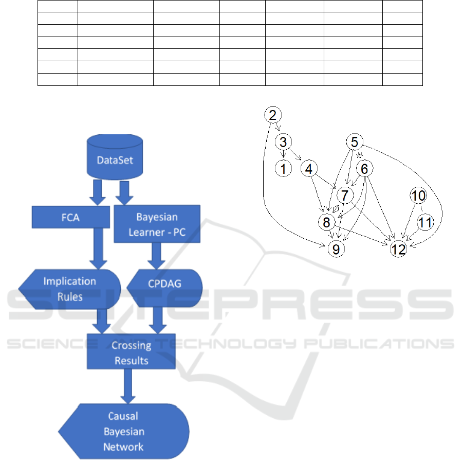
Table 2: Example: Formal Context.
Patient first.internment over.70.years T.over.4 over.2.hour Emergency ASA.2
P
1
X X X
P
2
X X X X
P
3
X X X X
P
4
X X X X X
P
5
X X X
P
6
X X
and FCA, the results were submitted for analysis of
an expert.
Figure 4: Methods.
The data set used in this article contains information
about 5,476 surgeries performed in 5 hospitals in the
city of Belo Horizonte - Brazil. It consists of 12 di-
chotomous (yes / no) attributes. Table 3 presents the
description of each random variable.
To generate the Bayesian Network, it was used PC
algorithm through R package pcalg (Kalisch et al.,
2012) and the IDE RStudio Version 1.0.136. PC was
applied to the data set and the output is shown in Fig.
5. The significance level (alpha) for individual condi-
tional independence tests, second stage described in
table 1, used in this paper was 0.05.
Figure 5: CPDAG Generated by PC.
Fig. 5 presents the resulting output, the equiva-
lence class (CPDAG), of PC algorithm. The resulting
CPDAG has 25 edges, 1 undirected, 2 bidirected and
22 directed edges.
The two bidirected edges are: 5 ↔ 6 and 7 ↔ 8;
the undirected is 10 − 11. This means that there are
8, 2
3
, candidates DAGs to become the true Causal
Bayesian Network.
The Concept Explorer (ConExp), a graphical tool
for Formal Concept Analysis, were used to extract im-
plication rules based on Duquenne-Guigues.
It was identified 78 implications rules on the data
set. From this set of rules only those involving bidi-
rected and undirected edges were considered. Table 4
shows the number of rules and records of each impli-
cation rule.
It is important to note that the left side of
the implication rule (premise) can be compound
by a set of attributes. Therefore, the number of
rules presented in Table 4 considers attributes
involved in the rules. For example, in the rule:
over.70.years General.anesthesia local.in f ection
→ In f ected.Surgery, General.anesthesia, attribute
number 6 in Fig 5, is part of a set of others attributes
that compounds the premise of the implication rule.
Thus this rule was computed for attribute 6.
Another observation from table 4 is that there is
no rule 7 → 8 and 10 → 11 and only six records are
affected by the rule 5 → 6.
ICEIS 2020 - 22nd International Conference on Enterprise Information Systems
120

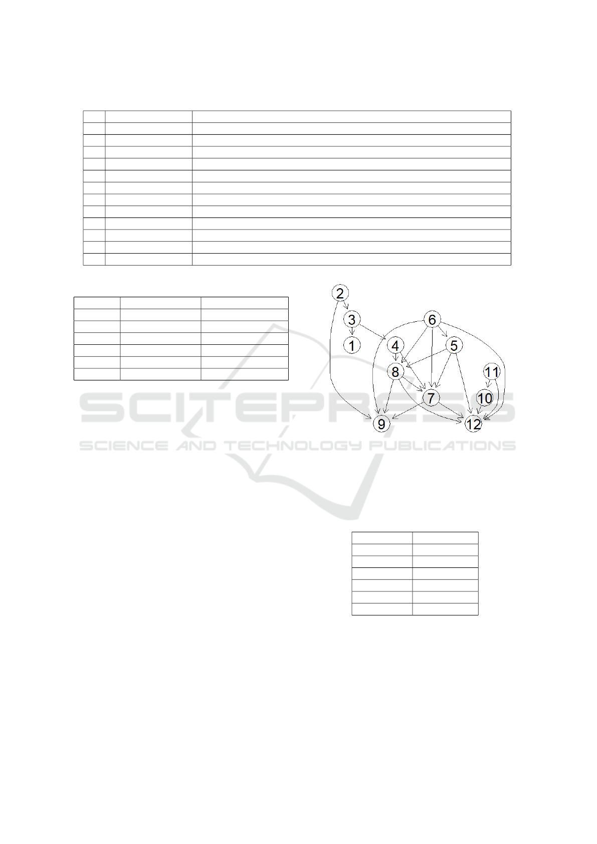
Table 3: Attributes Details.
Id Attributes Description
1 first.internment Indicates if it was the first internment of the patient.
2 over.70.years Indicates if the patient was over 70 years old.
3 T.over.4 Indicates if the patient has been hospitalized more than 4 days.
4 over.2.hours Indicates if the surgery lasted more than 2 hours.
5 Infected.Surgery Indicates if the surgery was infected.
6 General anesthesia Indicates if the patient was submitted to general anesthesia.
7 Emergency Indicates if it was an emergency surgery.
8 ASA.2 Indicates if ASA (American Society of Anesthesiologists) is greater than 2.
9 T.4 Indicates if the number of professionals involved in surgery is greater than 4.
10 global infection Indicates if patient had global infection.
11 local infection Indicates if patient had local infection.
12 death Indicates if patient gone to death.
Table 4: Attributes Implication.
Rule Number of Rules Number of records
5 → 6 6 6
6 → 5 13 365
7 → 8 0 0
8 → 7 9 22
10 → 11 0 0
11 → 10 5 40
Considering that there are no rules of attribute 7 im-
plying in 8 (7 → 8), neither rules that attribute 10
implies in 11 (10 → 11), edges between those nodes
were converted to unidirectional edges, 8 → 7 and
11 → 10.
Rule 5 → 6 represents only 0, 1% of all records
and rule 6 → 5, 6, 7%. It is important to highlight that
the attribute, 6, general anesthesia, appears as conse-
quent only in those 6 rules (see table 4). Attribute
5, Infected.Surgery, has 37 rules as consequent and
these 37 rules affect 572 instances. Therefore, 6 → 5
represents 69, 3% of all records affected by rules con-
taining attribute 6, General Anesthesia, as conclusion.
Considering the impact of the rules 5 → 6 and
6 → 5, shown in table 4, on the data set, the bi-
directed edge between nodes 6 and 5 were converted
to directed edge 6 → 5.
Applying the chances described before on the
CPDAG exhibited in Fig. 5, we obtain the DAG as
shown in Fig. 6.
In order to validate the resultant DAG (Fig. 6),
it was computed the causal effects (Table 5) of the
variables involved in the edges that were not directed
in Fig. 5. The causal effect was computed using do −
calculus as proposed by (Pearl, 2009).
In this paper interventions were made using the
IDA algorithm (Intervention calculus when the DAG
is Absent) (Kalisch et al., 2012) from pcalg package
Figure 6: True DAG.
of R. For each DAG of equivalence class, IDA esti-
mates the causal effect of x on y through a simple
linear regression lm(y x+ pa(x)) where pa(x) denotes
the parents of x in a DAG.
Table 5: Causal Effect.
Intervention Causal Effect
5 → 6 0.1349168
6 → 5 0.1557101
7 → 8 0.113705
8 → 7 0.1228783
10 → 11 0.9109589
11 → 10 0.9950096
From Table 5 it is possible to observe that causal ef-
fect of variable 6 on variable 5 is bigger than 5 on 6.
Also, the causal effect of 8 on 7 is bigger than 7 on 8
and causal effect of 11 on 10 is greater than 10 on 11.
Thus, it is expected that edges between those nodes
should be directed according to the greatest causal ef-
fects as shown in Fig. 6.
Undirected edges of the CPDAG (Fig. 5) using
An FCA-based Approach to Direct Edges in a Causal Bayesian Network: A Pilot Study using a Surgery Data Set
121

FCA and interventions were directed to the same di-
rections, this means that both approaches produced
the same causal DAG. Thus, it is possible to observe
that the interventions validate the results obtained us-
ing FCA.
The DAG shown in Fig. 6 is expected to be the
true causal network. In this sense, this DAG was pre-
sented to a specialist in order to validate its correct-
ness.
According to the expert, in a causal interpretation,
global infection does not cause local infection, be-
cause it is matter of temporal order. First come the
local infection and after global infection. Therefore,
the direction of the edge between nodes 10 and 11,
can only be 11 → 10.
Considering the bi-directed edge nodes 7 (Emer-
gency) and 8 (ASA), ASA is a classification, from 1 to
6, for assessing the health of the patient. The higher is
the number, worse is his health stands. Thus, there is a
relationship between these two attributes, which may
have a common cause or a relationship of causality
between them, once that how worse is patient’s con-
dition, more urgent became the surgery. For example,
according to (Aronson WL, 2003), in the original ver-
sion of ASA from 1941, ASA class 5 indicates ”Emer-
gencies that would otherwise be graded in Class 1 or
Class 2.”. Nowadays in each class of ASA is added a
letter E indicating if it is an emergency surgery or not.
Therefore, it is reasonable that the direction of the
edge between ASA and Emergency goes from ASA
to Emergency, not the opposite, once that ASA may
have direct effect on the emergency of the surgery, but
it is important to highlight that it is not the only factor
that influences the urgency of the surgery.
The relationship between attributes In-
fected.surgery (5) and general.anesthesia (6) is
correlated, according to the specialist, but it is not
possible to say that one causes another.
4 CONCLUSIONS
The main goal of this article was combining Causal
Inference and Formal Concept Analysis to establish
causality relationship between random variables. In
this sense we can conclude that, once causality re-
quires interventions or background knowledge to de-
fine the true DAG, FCA seems an alternative to help
in identifying the causal relationship.
Even if the implication rule does not necessarily
mean causality, it is useful in identifying relationships
among random variables through attribute implica-
tions. Therefore, the FCA can be used as a heuristic to
direct edges when the Bayesian learners’ algorithms
were unable to orient the edges between the vertices.
As future work, one should apply this heuristic in
other real applications using different type of data,
numerical for example, and create an algorithm that
combine these two theories, Causal Inference and
FCA. The researcher can also compare the results ob-
tained with others approaches of directing edges when
the true graph is unknown.
REFERENCES
Aronson WL, McAuliffe MS, M. K. (2003). Variability in
the american society of anesthesiologists physical sta-
tus classification scale. AANA Journal, 71(4):265–74.
Carpineto, C. and Romano, G. (2004). Concept Data Anal-
ysis: Theory and Applications. John Wiley &
Sons, Inc., USA.
de Carvalho, W. F. and Zarate, L. E. (2019). Causality re-
lationship among attributes applied in an educational
data set. In Proceedings of the 34th ACM/SIGAPP
Symposium on Applied Computing, SAC ’19, pages
1271–1277, New York, NY, USA. ACM.
Flesch, I. and Lucas, P. J. (2007). Markov Equivalence in
Bayesian Networks, pages 3–38. Springer Berlin Hei-
delberg, Berlin, Heidelberg.
Guyon, I. and Aliferis, C. F. (2007). Causal feature selec-
tion.
Hyttinen, A., Eberhardt, F., and J
¨
arvisalo, M. (2015). Do-
calculus when the true graph is unknown. In Proceed-
ings of the Thirty-First Conference on Uncertainty in
Artificial Intelligence, UAI’15, pages 395–404, Ar-
lington, Virginia, United States. AUAI Press.
Kalisch, M., M
¨
achler, M., Colombo, D., Maathuis, M., and
B
¨
uhlmann, P. (2012). Causal inference using graphi-
cal models with the r package pcalg. Journal of Sta-
tistical Software, Articles, 47(11):1–26.
ˇ
Skopljanac Ma
ˇ
cina, F. and Bla
ˇ
skovi
´
c, B. (2014). Formal
concept analysis – overview and applications. Proce-
dia Engineering, 69:1258 – 1267. 24th DAAAM In-
ternational Symposium on Intelligent Manufacturing
and Automation, 2013.
Neapolitan, R. E. (2003). Learning Bayesian Networks.
Prentice-Hall, Inc., Upper Saddle River, NJ, USA.
Pearl, J. (2009). Causality: Models, Reasoning and Infer-
ence. Cambridge University Press, New York, NY,
USA, 2nd edition.
Poelmans, J., Ignatov, D. I., Kuznetsov, S. O., and Dedene,
G. (2013). Formal concept analysis in knowledge pro-
cessing: A survey on applications. Expert Systems
with Applications, 40(16):6538 – 6560.
Shpitser, I., Mohan, K., and Pearl, J. (2015). Missing data
as a causal and probabilistic problem. In Proceedings
of the Thirty-First Conference on Uncertainty in Arti-
ficial Intelligence, UAI’15, pages 802–811, Arlington,
Virginia, United States. AUAI Press.
Spirtes, P., Glymour, C., and Scheines, R. (2000). Causa-
tion, Prediction, and Search. MIT press, 2nd edition.
ICEIS 2020 - 22nd International Conference on Enterprise Information Systems
122

Tsamardinos, I., Borboudakis, G., Katsogridakis, P.,
Pratikakis, P., and Christophides, V. (2019). A greedy
feature selection algorithm for big data of high dimen-
sionality. Machine Learning, 108(2):149–202.
Verma, T. and Pearl, J. (1991). Equivalence and synthesis
of causal models. In Proceedings of the Sixth Annual
Conference on Uncertainty in Artificial Intelligence,
UAI ’90, pages 255–270, New York, NY, USA. Else-
vier Science Inc.
Wille, R. (1982). Restructuring lattice theory: An approach
based on hierarchies of concepts. In Rival, I., edi-
tor, Ordered Sets, pages 445–470, Dordrecht. Springer
Netherlands.
Z
´
arate, L. E., Dias, S. M., and Song, M. J. (2008). Fcann:
A new approach for extraction and representation of
knowledge from ann trained via formal concept anal-
ysis. Neurocomputing, 71(13):2670 – 2684. Artificial
Neural Networks (ICANN 2006) / Engineering of In-
telligent Systems (ICEIS 2006).
An FCA-based Approach to Direct Edges in a Causal Bayesian Network: A Pilot Study using a Surgery Data Set
123