Towards a Comprehensive Model for the Impact of Traffic Patterns on
Air Pollution
Caterina Balzotti
1
, Maya Briani
2
, Barbara de Filippo
2
and Benedetto Piccoli
3
1
SBAI Department, Sapienza Universit
`
a di Roma, Rome, Italy
2
Consiglio Nazionale delle Ricerche, Istituto per le Applicazioni del Calcolo M. Picone, Rome, Italy
3
Department of Mathematical Sciences, Rutgers University, Camden, U.S.A.
Keywords:
Road Traffic Modeling, Second Order Traffic Model, Air Pollutant Emissions, Ozone Production.
Abstract:
The impact of vehicular traffic on society is huge and multifaceted, including economic, social, health and
environmental aspects. The problems is complex and hard to model since it requires to consider traffic pat-
terns, air pollutant emissions, and the chemical reactions and dynamics of pollutants in the low atmosphere.
This paper aims at exploring a comprehensive simulation tool ranging from vehicular traffic all the way to
environmental impact. As first step in this direction, we couple a traffic second-order model, tuned on NGSIM
data, with an nitrogen oxides (NO
x
) emission model and a set of equations for some of the main chemical
reactions behind ozone (O
3
) production.
1 INTRODUCTION
The impact of road traffic and its inefficiencies on so-
ciety is well known and was documented with quan-
titative estimates for more than a decade. In 2007,
in the sole US, traffic phenomena (such as conges-
tion) contributed for an economic loss of $78 billion.
The latter was estimated in the form of 4.2 billion lost
hours for delays and 2.9 billion gallons of wasted fuel
(TRB Executive Committee, 2013). Moreover, the so-
cietal impact is high also in terms of pollution and en-
vironmental effects, with road traffic accounting for
nearly one third of carbon dioxide (CO
2
) emissions
(TRB Executive Committee, 2011). While CO
2
is
probably one of the most studied molecules, the ef-
fect on health is also related to other pollutants, such
as particulate matters and nitrogen dioxide (NO
2
), see
(Zhang and Batterman, 2013). In this paper we focus
on the production of ozone (O
3
) which is strictly con-
nected with the NO
x
gases in the atmosphere (Atkin-
son, 2000; Wang et al., 2017; Chameides et al., 1988).
New technologies have the possibility of con-
tributing to reduce such heavy toll and even small
improvements (in relative terms) in this polluted ar-
eas will contribute to substantial economic and envi-
ronmental positive impact. Notice that much atten-
tion has been devoted in traffic literature to quantities
such as flow, capacity and travel time. However, ad-
vanced modeling of fuel consumption and emission
still faces limitations, especially for tools which can
be integrated with the increasing flow of data from
probe sensors. One of the main reasons is the high
variability of fuel consumption and emissions, which
are influenced by many factors as the vehicle type,
make, model, year and others.
Interestingly, traffic patterns, such as congestion
and traveling waves, account for large variations in
fuel consumption, and consequently emissions, but
smaller ones for flow and travel times. Therefore, im-
provement in terms of traffic patterns will mostly af-
fect fuel consumption and emissions, rather than trav-
eling times. For instance, it was shown via simulation
that a small number of autonomous and connected ve-
hicles may contribute to reduce the formation of traf-
fic waves and smooth traffic flow, see (Davis, 2004;
Talebpour and Mahmassani, 2016; Gu
´
eriau et al.,
2016; Wang et al., 2016; Knorr et al., 2012). More-
over, experimental evidence showed that this results
in significant reduction of fuel consumption and emis-
sions, see (Stern et al., 2018; Stern et al., 2019). A
key point is that many results show how even at very
low penetration (i.e. percentage of vehicles which are
autonomous or connected) the effect may be of great
significance. Similar benefits may be achieved by
improving driving efficiency, however this approach
needs the development of robust information flow to
the drivers or the use of specialized fleets.
Balzotti, C., Briani, M., de Filippo, B. and Piccoli, B.
Towards a Comprehensive Model for the Impact of Traffic Patterns on Air Pollution.
DOI: 10.5220/0009391502210228
In Proceedings of the 6th International Conference on Vehicle Technology and Intelligent Transport Systems (VEHITS 2020), pages 221-228
ISBN: 978-989-758-419-0
Copyright
c
 2020 by SCITEPRESS – Science and Technology Publications, Lda. All rights reserved
221

Despite this success, a comprehensive and ad-
vanced evaluation tool, which simulates benefits from
traffic regularization, is still lacking. Current es-
timates are mainly based on statistical analysis of
scarce sample data. However, a sound validation of
these results at large scale requires the development
of a comprehensive tool, which will model the vari-
ous aspects of the problem, ranging from traffic flow
all the way to evaluation of pollutant effects on the
environment. This paper aims at giving a first attempt
for the construction of such tool and provides a gen-
eral approach to connect traffic simulations to chemi-
cal reactions.
2 A MODULAR APPROACH TO
EVALUATE TRAFFIC IMPACT
We propose a modular approach as shown in Figure
1.
Figure 1: A Schematic Representation of the Modular Ap-
proach.
The modules are the following:
• Traffic simulator
• Fuel consumption and emissions model
• Chemical reactions model
• Diffusion and transportation model
• Impact evaluation module (e.g. monument degra-
dation, health impact, other)
The first module aims at simulating the load of a road
network on a given time scale, which can range from
few hours to weeks. We propose to use macroscopic
traffic models, described in detail in Section 3, which
can be fed by mobile sensors data (Work et al., 2010).
The second module will be based on the use of pol-
lutant emission rate estimators, which can use mea-
surements and data produced by module one for ag-
gregated estimates, see (Piccoli et al., 2015). The
third module needs to be developed in dependence of
the considered pollutants, while the fourth is based
on reaction-diffusion models using partial differen-
tial equations (Alvarez-V
´
azquez et al., 2017; Sama-
ranayake et al., 2014). Finally, last module is highly
dependent on the considered impact.
In this paper, we focus on the first three modules,
aiming to give a possible approach to evaluate the im-
pact of vehicular traffic on the production of ozone.
3 TRAFFIC MODEL
Depending on the scale at which traffic models rep-
resent vehicular traffic, they are divided in the fol-
lowing categories: cellular, each road is represented
by cells which may contain more vehicles (Nagel
and Schreckenberg, 1992; Fukui and Ishibashi, 1996;
Daganzo, 2006; Sakai et al., 2006; Alperovich and
Sopasakis, 2008); microscopic, individual vehicles
dynamics are modeled by ordinary differential equa-
tions (Pipes, 1953; Newell, 1961; Bando et al., 1995)
and continuum, where the car density evolves accord-
ing to a partial differential equation, which can be of
kinetic type (Herman and Prigogine, 1971; Phillips,
1979; Klar and Wegener, 2000; Illner et al., 2003)
or fluid-dynamic ones (Lighthill and Whitham, 1955;
Richards, 1956; Kerner and Konh
¨
auser, 1993; Kerner
and Konh
¨
auser, 1994; Aw and Rascle, 2000). For a
deeper review see (Helbing, 2001; Albi et al., 2019;
Garavello et al., 2016; Piccoli and Tosin, 2011).
The different classes of models have advan-
tages and disadvantages. We focus on macroscopic
fluid-dynamic ones. Such models are based on the
conservation of vehicles, ρ
t
+(ρv)
x
= 0, where ρ(x,t)
is the vehicle density and v(x,t) the average velocity.
The first order Lighthill-Whitham-Richards (LWR)
model (Lighthill and Whitham, 1955; Richards,
1956) assumes a functional relationship between
velocity and density, v = v(ρ), and yields the LWR
PDE
ρ
t
+ f (ρ)
x
= 0 , (1)
where f = ρv(ρ) is the flow rate of vehicles. Second
order models consider ρ and v as independent quanti-
ties and consist of balance laws
(
ρ
t
+ (ρv)
x
= 0
v
t
+ f (ρ,v)
x
= A(ρ,v),
(2)
where A is an acceleration term. Among the most
used models we recall the Aw-Rascle-Zhang (ARZ)
model (Aw and Rascle, 2000; Greenberg, 2001;
Zhang, 2002). These models are able to capture the
formation of traffic waves from steady traffic situ-
ations (known also as phantom traffic jams) which
are observed experimentally (Sugiyama et al., 2008).
Such waves are responsible for breaking events, the
increase in fuel consumption and many other draw-
backs with environmental effects. For these reasons
in this paper we adopt second order models to simu-
late complex traffic situations which are the main re-
sponsible of pollutant emissions.
Specifically, we use the second order Collapsed
Generalized Aw-Rascle-Zhang (CGARZ) model (Fan
et al., 2017; Fan, 2013), to describe the evolution
of traffic flow. The CGARZ model belongs to the
VEHITS 2020 - 6th International Conference on Vehicle Technology and Intelligent Transport Systems
222

family of macroscopic Generic Second Order Mod-
els (GSOM) (Lebacque et al., 2007), which satisfy
(
ρ
t
+ (ρv)
x
= 0
w
t
+ vw
x
= 0,
with v = V (ρ,w),
(3)
for a specific velocity function V . Here ρ(x,t) is the
traffic density, v(x,t) the velocity and and w(x,t) is
a property of vehicles which is advected by traffic
flow. GSOM are characterized by a family of fun-
damental diagrams f (ρ,w) = ρV (ρ, w), parametrized
by w. The peculiarity of the CGARZ model is that
it possesses a single-valued fundamental diagram in
free-flow, and a multi-valued function in congestion.
Here, we use the flux and velocity functions proposed
in (Balzotti et al., 2019).
4 EMISSIONS
In this section we introduce an emission model suit-
able for several air pollutants. Specifically, we focus
on ozone (O
3
) and nitrogen oxides (NO
x
) which are of
particular interest in areas with heavy vehicular traffic
and high amounts of UV radiation. Ozone is a sec-
ondary pollutant and its production is due to a com-
plex system of reactions of its precursors, mainly NO
x
gases, in a sunlight ambient, (Jacob, 2000; Song et al.,
2011).
Starting from the model proposed in (Panis et al.,
2006), we assume to have N vehicles in a stretch of
road going all at the same speed ¯v, with the same ac-
celeration ¯a. Then, the emission rate E(t) at time t is
given by the N contributes of the vehicles, such that
E(t) = N max{E
0
, f
1
+ f
2
¯v(t) + f
3
¯v(t)
2
+ f
4
¯a(t) + f
5
¯a(t)
2
+ f
6
¯v(t) ¯a(t)},
(4)
where E
0
is a lower-bound of emission and f
1
to f
6
are emission constants. See (Panis et al., 2006, Table
2) for the NO
x
estimated coefficients. In this work,
the velocity and acceleration quantities in equation (4)
are provided by the numerical solution to the CGARZ
model (3). We refer to (Balzotti et al., 2019) for the
validation of the proposed approach.
5 CHEMICAL REACTIONS
In this section we are interested in the main chem-
ical reactions of nitrogen oxides which lead to the
production of ozone. Ozone is produced in the tro-
posphere by a complex reaction mechanism that in-
volves mainly volatile organic compounds and NO
x
(Jacob, 2000). Nitrogen oxides is a collective term
used to refer to nitrogen oxide (NO) and nitrogen
dioxide (NO
2
), that are usually produced from fuel
combustion in car engines, especially at high temper-
atures (Omidvarborna et al., 2015). Classified as a
secondary pollutant, NO
2
is a very reactive compound
that can be photo-dissociated and produce atomic
oxygen (O) that quickly combines with an oxygen
molecule to form an ozone molecule. This complex
mechanism is considered one of key steps in the for-
mation of ground-level ozone. In polluted regions
with high vehicle emissions, NO
2
is a relevant pre-
cursor substance for the ozone in photochemical smog
and the ozone production is due to the following re-
actions
NO
2
+ hν −→ O + NO (5)
O + O
2
+ M −→ O
3
+ M, (6)
where h is Planck’s constant and ν the frequency. M is
a chemical species, such as oxygen (O
2
) or nitrogen
(N
2
), that adsorbs the excess of energy generated in
reaction (6), (Manahan, 2017). Moreover, in presence
of NO, O
3
reacts with it and this reaction destroys the
ozone and reproduces the NO
2
,
O
3
+ NO −→ O
2
+ NO
2
. (7)
This means that the previous reactions do not result
in net ozone production, indeed reactions (6) and (7)
balance the cycle between NO
x
and O
3
. The com-
plexity of the ground-level ozone production, that in-
volves many different precursors such as VOC, NO
x
and others, forces us to focus on a simple subset of
chemical reactions not taking into account important
aspects such as diurnal/nocturnal variation and their
relative dispersion, see (Song et al., 2011).
5.1 Estimating the Production of O
3
In this section we define a model consisting in as
system of ordinary differential equation to represent
the ozone production resulting from traffic emissions.
More precisely, we set up ordinary differential equa-
tions for each of the chemical reactions introduced in
(5), (6) and (7). We denote the chemical species con-
centration by [·] = [weight unit/volume unit].
We assume that the first reaction (5) takes place
only during the daily hours with a fixed kinetic con-
stant k
1
. Thus the associated system of ODE is
d[NO
2
]
dt
= −k
1
[NO
2
]
d[O]
dt
= k
1
[NO
2
]
d[NO]
dt
= k
1
[NO
2
].
(8)
Towards a Comprehensive Model for the Impact of Traffic Patterns on Air Pollution
223

For the second reaction (6) we choose M to be O
2
,
then
O + 2O
2
−→ O
3
+ O
2
and we call k
2
the associated kinetic constant. We
obtain the system
d[O]
dt
= −k
2
[O] [O
2
]
2
d[O
2
]
dt
= −k
2
[O] [O
2
]
2
d[O
3
]
dt
= k
2
[O] [O
2
]
2
.
(9)
The third reaction (7) gives us the third system of
ODEs with kinetic constant k
3
d[O
3
]
dt
= −k
3
[O
3
] [NO]
d[NO]
dt
= −k
3
[O
3
] [NO]
d[O
2
]
dt
= k
3
[O
3
] [NO]
d[NO
2
]
dt
= k
3
[O
3
] [NO].
(10)
Finally, we combine the systems (8), (9) and (10)
into a unique set of equations, adding the contribution
of the traffic emissions. We assume that the reactions
take place in a volume of dimension ∆x
3
, and the traf-
fic emissions contribution acts as a source term for the
concentration of NO and NO
2
. Hence, we define the
variation of the concentration of NO
x
in ∆x
3
, at each
time t as
S
NO
x
=
E
NO
x
(t)
∆x
3
, (11)
where the emission rate E
NO
x
(t) is given by (4). The
final system then becomes
d[O]
dt
= −k
2
[O] [O
2
]
2
+ k
1
[NO
2
]
d[O
2
]
dt
= −k
2
[O] [O
2
]
2
+ k
3
[O
3
] [NO]
d[O
3
]
dt
= k
2
[O] [O
2
]
2
− k
3
[O
3
] [NO]
d[NO]
dt
= k
1
[NO
2
] − k
3
[O
3
] [NO]
+(1 − p)S
NO
x
d[NO
2
]
dt
= −k
1
[NO
2
] + k
3
[O
3
] [NO]
+pS
NO
x
,
(12)
where p is the percentage of NO
2
derived from the
emission rate of NO
x
.
6 NUMERICAL TESTS
In this section we give some tests to illustrate how the
first three modules in Figure 1 are combined to esti-
mate the production of ozone.
Let us start by considering the CGARZ traffic model
(3) on a road parametrized by the interval [0,L] on a
time horizon [0,T ]. We assume a constant left bound-
ary condition ρ(0,t) = u
0
, ∀ t ∈ [0,T ], and we allow
all vehicles to leave the road on the right. The pa-
rameters used in all simulations are T = 30 min, L =
10km, maximum vehicles velocity allowed V
max
=
120km/h, road capacity ρ
max
= 133 veh/km, u
0
=
42veh/km and the initial density ρ
0
is
ρ
0
(x) =
(
42 0 ≤ x ≤ `
110 ` < x ≤ L
(13)
with ` = 4.5km.
6.1 From Traffic Quantities to NO
x
Emissions
We divide our domain into cells, with space step ∆x
and time step ∆t. For each cell centered at x
j
and time
t
n
of the numerical grid, we compute the vehicles den-
sity ρ
n
j
and speed V
n
j
using the Godunov-type second
order cell transmission scheme (Fan et al., 2017) to
solve the CGARZ system (3).
To estimate the NO
x
emission rate (4), we need to
compute the acceleration of vehicles. Following the
approach proposed in (Luspay et al., 2010; Zegeye
et al., 2013), which distinguishes between the tem-
poral acceleration and the spatial-temporal accelera-
tion, we apply the resulting acceleration formula
A
k
i
=
V
k+1
i
−V
k
i
∆t
+V
k
i
V
k+1
i+1
−V
k+1
i
∆x
. (14)
We set now ∆x = 0.1km and ∆t = 0.5∆x/V
max
and
starting by initial data (13) we have a traffic dynamic
described by a shock wave which propagates back-
ward from the middle of the road, until the interaction
with the rarefaction wave stemming from the right,
changes the shock speed to positive. The correspond-
ing variation in time of the total emission of NO
x
,
defined as the sum on the cells of the NO
x
emission
rates, increases until the traffic dynamic is represented
by the shock wave and then it starts to decrease to its
lower-bound defined by null acceleration.
We are now interested in studying the effects of
traffic lights on the previous dynamic. Specifically,
we test the impact on NO
x
emissions of different
traffic light cycles varying the time frame of the red
phase, which corresponds to a condition that imposes
VEHITS 2020 - 6th International Conference on Vehicle Technology and Intelligent Transport Systems
224

vanishing outflow on the right boundary of the do-
main. Let t
g
and t
r
be the time of the green and red
traffic light phase respectively. To show the influences
of traffic lights on NO
x
emissions, we vary t
g
and t
r
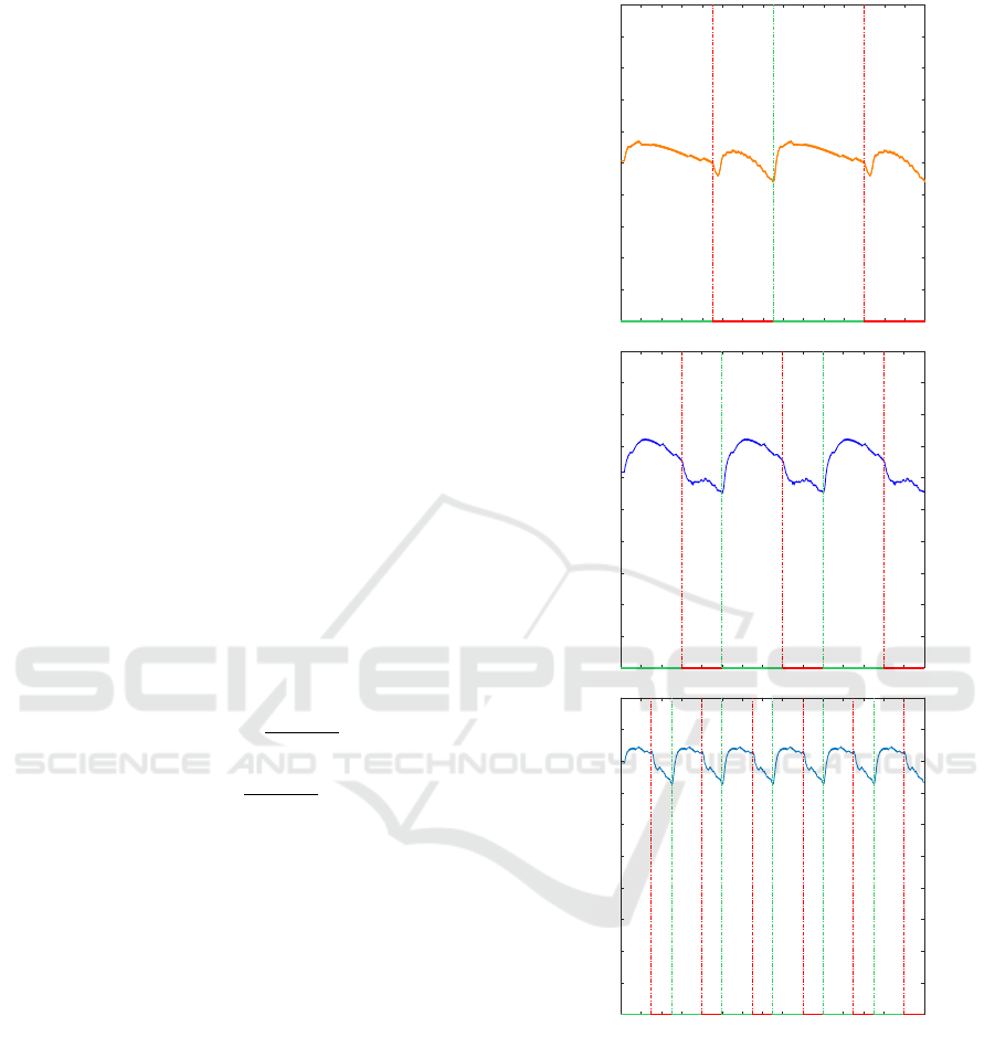
fixing their ratio to 3/2. In Figure 2 we show the NO
x
emissions during 15 minutes of traffic light on. In par-
ticular, on the top we set t
g
= 4.5 min and t
r
= 3 min,
in the center t
g
= 3min and t
r
= 2min and on the bot-
tom t
g
= 1.5 min and t
r
= 1 min. We observe that the
duration of the traffic light t
g
+ t
r
has an high influ-
ence on the maximum value of the total NO
x
emission
rate, indeed it grows with the increase of the vehicles
restarts.
6.2 Production of Ozone
In this section we use system (12) to estimate the con-
centration of ozone along the entire road. Following
(Jacobson, 2005), we fix the reaction rate parameters
as k
1
= 0.02 s
−1
, k
2
= 6.09×10
−34
cm
6
/molecule and
k
3
= 1.81 ×10
−14
cm
3
/molecule.
For each cell x
j
, we set the initial concentrations
as:
[O] = [O
3
] = 0,
[O
2
] = 5.02 × 10
18
molecule/cm
3
,
and, for NO and NO
2
we use the relation (11) such
that at the initial time t = 0
[NO] = (1 − p)
E
NO
x
(0)
∆x
3
,
[NO
2
] = p
E
NO
x
(0)
∆x
3
,
with p = 0.15 according to (Carslaw et al., 2011).
For each time step n, we then compute the source
term (11) due to traffic by using the NO
x
emission rate
obtained in the previous tests cases with and without
traffic lights, and we solve the ODEs system (12) in
each cell x
j
.
In Figure 3, we show the O
3
evolution along the
entire road, during 15 minutes of simulation. As to be
expected, we observe a different behavior in presence
or not of the traffic lights and a higher O
3
concentra-
tion with traffic light on.
In Figure 4 we compare the variation in time of
the total concentration of O
3
in the case of dynamic
without traffic lights with the case with traffic light on
defined by t
g
= 3 min and t
r
= 2 min. As expected, the
ozone concentration is amplified by the presence of
the traffic lights.
6.3 Weekly Ozone Production
In this section we estimate the production of ozone
and of the other chemical species during a whole
15 20 25 30
Time (minute)
2800
2900
3000
3100
3200
3300
3400
3500
3600
3700
3800
NO
x
emission rate (g/h)
15 20 25 30
Time (minute)
2800
2900
3000
3100
3200
3300
3400
3500
3600
3700
3800
NO
x
emission rate (g/h)
15 20 25 30
Time (minute)
2800
2900
3000
3100
3200
3300
3400
3500
3600
3700
3800
NO
x
emission rate (g/h)
Figure 2: Variation in Time of the Total NO
x
Emission Rate
along the Entire Road with t
g
/t
r
= 3/2 and Varying the
Traffic Light Duration: (Top) t
g
= 4.5 min and t
r
= 3 min;
(Center) t
g
= 3 min and t
r
= 2 min; (Bottom) t
g
= 1.5 min
and t
r
= 1 min.
week. Day and night are simulated by varying the
kinetic constant k
1
associated to reaction (5) which
represents the photo-dissociation of NO
2
by sunlight.
The results of our model are to be taken with care be-
cause, as noticed above, we did not include all com-
plex chemical reactions happening in the atmosphere.
In particular we can not use such results to compare
Towards a Comprehensive Model for the Impact of Traffic Patterns on Air Pollution
225

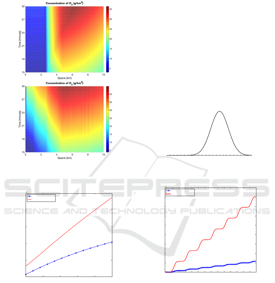
Figure 3: O
3
Evolution along the Entire Road, for 15min
of Simulation, in the Case of Dynamics without (Top) and
with (Bottom) Traffic Light.
15 18 21 24 27 30
Time (minute)
1.5
2
2.5
3
3.5
4
Concentration (g/km
3
)
10
3
Concentration of O
3
(g/km
3
)
Without traffic light
With traffic light
Figure 4: Variation in Time of the Total Concentration of
O
3
in the Case of Dynamics with (Red-Solid) and without
(Blue-Circles) Traffic Light.
with data from air pollution sensors. However, our
scope is to compare production of NO
x
and O
3
as due
to different traffic patterns. So our analysis is intended
a first step in understanding the impact on pollution
of traffic lights. In Figure 5 we show the hypothetical
trend of parameter k
1
as a Gaussian function of time.
We then solve system (12) assuming that the source
term S
NO
x
due to traffic has a similar trend of k
1
dur-
ing day and night, see again Figure 5. Specifically,
the maximum of S
NO
x
is computed by the mean of the
values during its periodical trend when traffic lights
on (see Figure 2).
To further investigate the impact of the traffic light
on emissions, we compute the weekly total amount of
the considered chemical species. In Figures 6 and 7
we compare the concentration in presence of the traf-
fic light (red-solid line) with respect to the one ob-
tained in the case without traffic light (blue-circles
line) for NO and NO
2
respectively. We observe that
NO and NO
2
productions are highly amplified by the
presence of the traffic light. The dynamic of O
3
is dif-
ferent, since it reaches its saturation value each day at
3 p.m. (in accordance to the time in which the param-
eter k
1
in Figure 5 is maximum) regardless the pres-
ence or not of the traffic light.
0 1 2 3 4 5 6 7 8 9 10 11 12 13 14 15 16 17 18 19 20 21 22 23 24
Time (h)
Figure 5: Daily Hypothetical Trend of Parameter k
1
and of
the Source Term S
NO
x
as a Function of Time.
0 1 2 3 4 5 6 7
Day
0
2
4
6
8
10
12
14
16
18
10
7
Concentration of NO (g/km
3
)
Without traffic light
With traffic light
Figure 6: Total Production of NO Due to Traffic during a
Whole Week with (Red-Solid) and without (Blue-Circles)
Traffic Light.
7 CONCLUSIONS
The impact of air quality on public health is one of
the world’s worst open problems. Emissions from
vehicles is one of the major source of the detected
air pollutants. In this paper we coupled a CGARZ
second-order traffic model with an estimator for NO
x
emission rate and a system of equations representing
some of the main chemical reactions responsible for
VEHITS 2020 - 6th International Conference on Vehicle Technology and Intelligent Transport Systems
226

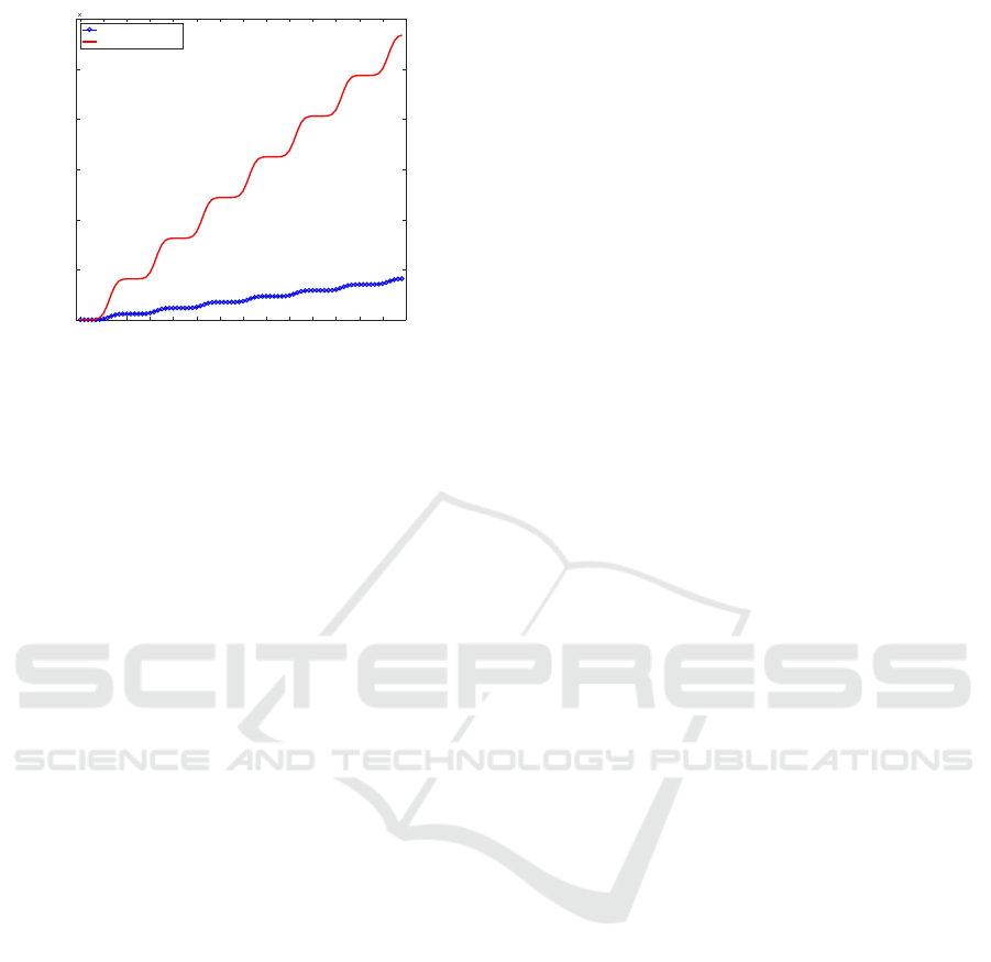
0 1 2 3 4 5 6 7
Day
0
5
10
15
20
25
30
10
6
Concentration of NO
2
(g/km
3
)
Without traffic light
With traffic light
Figure 7: Total Production of NO
2
Due to Traffic during a
Whole Week with (Red-Solid) and without (Blue-Circles)
Traffic Light.
the ozone production. Future investigations will in-
clude pollutant diffusion and transportation in the air
and other chemical reactions. Moreover, we aim at
extending the tool to road network to better capture
environmental effects.
REFERENCES
Albi, G., Bellomo, N., Fermo, L., Ha, S.-Y., Kim, J.,
Pareschi, L., Poyato, D., and Soler, J. (2019). Ve-
hicular traffic, crowds, and swarms: from kinetic the-
ory and multiscale methods to applications and re-
search perspectives. Math. Models Methods Appl.
Sci., 29(10):1901–2005.
Alperovich, T. and Sopasakis, A. (2008). Modeling high-
way traffic with stochastic dynamics. J. Stat. Phys,
133:1083–1105.
Alvarez-V
´
azquez, L. J., Garc
´
ıa-Chan, N., Mart
´
ınez, A., and
V
´
azquez-M
´
endez, M. E. (2017). Numerical simula-
tion of air pollution due to traffic flow in urban net-
works. J. Comput. Appl. Math., 326:44–61.
Atkinson, R. (2000). Atmospheric chemistry of VOCs and
NO
x
. Atmos. Environ., 34(12–14):2063–2101.
Aw, A. and Rascle, M. (2000). Resurrection of “Second
Order” Models of Traffic Flow. SIAM J. Appl. Math.,
60:916–944.
Balzotti, C., Briani, M., De Filippo, B., and Piccoli, B.
(2019). Evaluation of NO
x
emissions and ozone pro-
duction due to vehicular traffic via second-order mod-
els. arXiv preprint arXiv:1912.05956.
Bando, M., Hesebem, K., Nakayama, A., Shibata, A., and
Sugiyama, Y. (1995). Dynamical model of traffic
congestion and numerical simulation. Phys. Rev. E,
51(2):1035–1042.
Carslaw, D. C., Beevers, S. D., Tate, J. E., Westmore-
land, E. J., and Williams, M. L. (2011). Recent ev-
idence concerning higher NO
x
emissions from pas-
senger cars and light duty vehicles. Atmos. Environ.,
45(39):7053–7063.
Chameides, W. L., Lindsay, R. W., Richardson, J., and
Kiang, C. S. (1988). The role of biogenic hydrocar-
bons in urban photochemical smog: Atlanta as a case
study. Science, 241(4872):1473–1475.
Daganzo, C. F. (2006). In traffic flow, cellular automata =
kinematic waves. Transp. Res. B, 40:396–403.
Davis, L. (2004). Effect of adaptive cruise control systems
on traffic flow. Physical Review E, 69(6):066110.
Fan, S. (2013). Data-Fitted Generic Second Order Macro-
scopic Traffic Flow Models. Ph.D. Thesis, Temple
University.
Fan, S., Sun, Y., Piccoli, B., Seibold, B., and Work,
D. B. (2017). A Collapsed Generalized Aw-Rascle-
Zhang Model and its Model Accuracy. arXiv preprint
arXiv:1702.03624.
Fukui, M. and Ishibashi, Y. (1996). Traffic Flow in 1D Cel-
lular Automaton Model Including Cars Moving with
High Speed. J. Phys. Soc. Japan, 65(6):1868–1870.
Garavello, M., Han, K., and Piccoli, B. (2016). Models for
Vehicular Traffic on Networks. American Institute of
Mathematical Sciences.
Greenberg, J. M. (2001). Extension and amplification of the
Aw-Rascle model. SIAM J. Appl. Math., 63:729–744.
Gu
´
eriau, M., Billot, R., El Faouzi, N.-E., Monteil, J.,
Armetta, F., and Hassas, S. (2016). How to assess the
benefits of connected vehicles? A simulation frame-
work for the design of cooperative traffic manage-
ment strategies. Transp. Res. Part C Emerg. Technol.,
67:266–279.
Helbing, D. (2001). Traffic and related self-driven many-
particle systems. Rev. Mod. Phys., 73:1067–1141.
Herman, R. and Prigogine, I. (1971). Kinetic theory of ve-
hicular traffic. Elsevier, New York.
Illner, R., Klar, A., and Materne, T. (2003). Vlasov-Fokker-
Planck Models for Multilane Traffic Flow. Commun.
Math. Sci., 1(1):1–12.
Jacob, D. J. (2000). Heterogeneous chemistry and tropo-
spheric ozone. Atmos. Environ., 34(12):2131–2159.
Jacobson, M. Z. (2005). Fundamentals of Atmospheric
Modeling. Cambridge University Press.
Kerner, B. S. and Konh
¨
auser, P. (1993). Cluster effect
in initially homogeneous traffic flow. Phys. Rev. E,
48:R2335–R2338.
Kerner, B. S. and Konh
¨
auser, P. (1994). Structure and
parameters of clusters in traffic flow. Phys. Rev. E,
50:54–83.
Klar, A. and Wegener, R. (2000). Kinetic Derivation of
Macroscopic Anticipation Models for Vehicular Traf-
fic. SIAM J. Appl. Math., 60(5):1749–1766.
Knorr, F., Baselt, D., Schreckenberg, M., and Mauve, M.
(2012). Reducing traffic jams via VANETs. IEEE
Transactions on Vehicular Technology, 61(8):3490–
3498.
Lebacque, J.-P., Mammar, S., and Haj-Salem, H. (2007).
Generic second order traffic flow modelling. In All-
sop, R. E., Bell, M. G. H., and Heydecker, B. G., ed-
itors, Transportation and Traffic Theory, Proc. of the
17th ISTTT, pages 755–776. Elsevier.
Towards a Comprehensive Model for the Impact of Traffic Patterns on Air Pollution
227

Lighthill, M. J. and Whitham, G. B. (1955). On kinematic
waves II. A theory of traffic flow on long crowded
roads. Proc. Roy. Soc. A, 229(1178):317–345.
Luspay, T., Kulcsar, B., Varga, I., Zegeye, S. K., De Schut-
ter, B., and Verhaegen, M. (2010). On acceleration
of traffic flow. In Proceedings of the 13th Interna-
tional IEEE Conference on Intelligent Transportation
Systems (ITSC 2010), pages 741–746. IEEE.
Manahan, S. (2017). Environmental chemistry. CRC press.
Nagel, K. and Schreckenberg, M. (1992). A cellular au-
tomaton model for freeway traffic. J. Phys. I France,
2:2221–2229.
Newell, G. F. (1961). Nonlinear Effects in the Dynamics of
Car Following. Oper. Res., 9(2):209–229.
Omidvarborna, H., Kumar, A., and Kim, D.-S. (2015).
NO
x
emissions from low-temperature combustion of
biodiesel made of various feedstocks and blends. Fuel
Process. Technol., 140(Supplement C):113 – 118.
Panis, L. I., Broekx, S., and Liu, R. (2006). Modelling in-
stantaneous traffic emission and the influence of traffic
speed limits. Sci. Total Environ., 371(1-3):270–285.
Phillips, W. F. (1979). A kinetic model for traffic flow with
continuum implications. Transportation Planning and
Technology, 5(3):131–138.
Piccoli, B., Han, K., Friesz, T. L., Yao, T., and Tang, J.
(2015). Second-order models and traffic data from
mobile sensors. Transp. Res. Part C Emerg. Technol.,
52(Supplement C):32 – 56.
Piccoli, B. and Tosin, A. (2011). Vehicular Traffic: A
Review of Continuum Mathematical Models, pages
1748–1770. Springer New York, New York, NY.
Pipes, L. A. (1953). An Operational Analysis of Traffic
Dynamics. J. Appl. Phys., 24:274–281.
Richards, P. I. (1956). Shock Waves on the Highway. Oper.
Res., 4(1):42–51.
Sakai, S., Nishinari, K., and Iida, S. (2006). A new stochas-
tic cellular automaton model on traffic flow and its
jamming phase transition. J. Phys. A: Math. Gen.,
39:15327–15339.
Samaranayake, S., Glaser, S., Holstius, D., Monteil, J.,
Tracton, K., Seto, E., and Bayen, A. (2014). Real-
Time Estimation of Pollution Emissions and Disper-
sion from Highway Traffic. Comput.-Aided Civ. Inf.,
29(7):546–558.
Song, F., Shin, J. Y., Jusino-Atresino, R., and Gao, Y.
(2011). Relationships among the springtime ground–
level NO
x
, O
3
and NO
3
in the vicinity of highways in
the US East Coast. Atmos. Pollut. Res., 2(3):374–383.
Stern, R., Cui, S., Delle Monache, M. L., Bhadani, R.,
Bunting, M., Churchill, M., Hamilton, N., Haulcy,
R., Pohlmann, H., Wu, F., Piccoli, B., Seibold, B.,
Sprinkle, J., and Work, D. B. (2018). Dissipation
of stop-and-go waves via control of autonomous ve-
hicles: Field experiments. Transp. Res. Part C Emerg.
Technol., 89:205–221.
Stern, R. E., Chen, Y., Churchill, M., Wu, F.,
Delle Monache, M. L., Piccoli, B., Seibold, B., Sprin-
kle, J., and Work, D. B. (2019). Quantifying air qual-
ity benefits resulting from few autonomous vehicles
stabilizing traffic. Transp. Res. Part D, 67:361–365.
Sugiyama, Y., Fukui, M., Kikuchi, M., Hasebe, K.,
Nakayama, A., Nishinari, K., Tadaki, S., and Yukawa,
S. (2008). Traffic jams without bottlenecks – Exper-
imental evidence for the physical mechanism of the
formation of a jam. New J. Phys., 10:033001.
Talebpour, A. and Mahmassani, H. S. (2016). Influence
of connected and autonomous vehicles on traffic flow
stability and throughput. Transp. Res. Part C Emerg.
Technol., 71:143–163.
TRB Executive Committee (2011). Special Report 307:
Policy Options for Reducing Energy and Greenhouse
Gas Emissions from U.S. Transportation. Technical
report, Transportation Research Board of the National
Academies.
TRB Executive Committee (2013). Critical issues in trans-
portation 2013. Technical report, Transportation Re-
search Board of the National Academies.
Wang, M., Daamen, W., Hoogendoorn, S. P., and van Arem,
B. (2016). Cooperative car-following control: Dis-
tributed algorithm and impact on moving jam features.
IEEE Transactions on Intelligent Transportation Sys-
tems, 17(5):1459–1471.
Wang, T., Xue, L., Brimblecombe, P., Lam, Y., Li, L.,
and Zhang, L. (2017). Ozone pollution in China: A
review of concentrations, meteorological influences,
chemical precursors, and effects. Sci. Total Environ.,
575:1582–1596.
Work, D., Blandin, S., Tossavainen, O.-P., Piccoli, B., and
Bayen, A. (2010). A traffic model for velocity data
assimilation. Appl. Math. Res. Express., 2010(1):1–
35.
Zegeye, S., De Schutter, B., Hellendoorn, J., Breunesse, E.,
and Hegyi, A. (2013). Integrated macroscopic traffic
flow, emission, and fuel consumption model for con-
trol purposes. Transp. Res. Part C Emerg. Technol.,
31:158–171.
Zhang, H. M. (2002). A non-equilibrium traffic model de-
void of gas-like behavior. Transp. Res. B, 36:275–290.
Zhang, K. and Batterman, S. (2013). Air pollution and
health risks due to vehicle traffic. Sci. Total Environ.,
450-451(Supplement C):307 – 316.
VEHITS 2020 - 6th International Conference on Vehicle Technology and Intelligent Transport Systems
228