Particle Swarm Optimization for Performance Management in

Multi-cluster IoT Edge Architectures

Shelernaz Azimi

, Claus Pahl

and Mirsaeid Hosseini Shirvani

Free University of Bozen-Bolzano, Bolzano, Italy

Department of Computer Engineering, Sari branch, Islamic Azad University, Sari, Iran

Keywords:

Internet of Things, Edge Computing, Cloud Computing, Particle Swarm Optimization, PSO, Performance.

Abstract:

Edge computing extends cloud computing capabilities to the edge of the network, allowing for instance

Internet-of-Things (IoT) applications to process computation more locally and thus more efﬁciently. We aim

to minimize latency and delay in edge architectures. We focus on an advanced architectural setting that takes

communication and processing delays into account in addition to an actual request execution time in a per-

formance engineering scenario. Our architecture is based on multi-cluster edge layer with local independent

edge node clusters. We argue that particle swarm optimisation as a bio-inspired optimisation approach is an

ideal candidate for distributed load processing in semi-autonomous edge clusters for IoT management. By

designing a controller and using a particle swarm optimization algorithm, we can demonstrate that processing

and propagation delay and the end-to-end latency (i.e., total response time) can be optimized.

1 INTRODUCTION

Edge computing provides an intermediate layer for

computation and storage at the ’edge’ of the network,

often between Internet-of-Things devices and central-

ized data center clouds (Mahmud et al., 2019; Pahl

et al., 2018). Edge computing promises better per-

formance through lower latency since computation is

moved closer to application. Reducing data transfer

time by avoiding the transfer of large volumes of data

to remote clouds has also the effect of reducing secu-

rity risks. Localization is here the key principle.

Performance and load management in edge archi-

tectures has been addressed in the past (Baktyan and

Zahary, 2018; Minh et al., 2019), but often the ar-

chitectures referred to do not reﬂect the often geo-

graphically distributed nature of edge computing. We

expand here on works like (Gand et al., 2020; Tata

et al., 2017) that have considered single autonomous

clusters only. We propose here a solution for a multi-

cluster solution, where each cluster operates semi-

autonomously, only being coordinated by an orches-

trator that manages load distribution. Another direc-

tion that we add is a realistic reﬂection of performance

concerns. In our performance model, we consider de-

lays caused by communication and queueing (prop-

agation delays) as well as processing delays of con-

trollers and edge execution nodes into a comprehen-

sive end-to-end latency concept that realizes the re-

sponse time from the requestor’s perspective.

Thus, our approach extends the state-of-the-art by

combining an end-to-end latency optimization frame-

work with a multi-cluster edge architecture. We pro-

pose Particle Swarm Optimization (PSO) for the op-

timization here. PSO is a bio-inspired evolutionary

optimization method (Saboori et al., 2008) to coordi-

nate between autonomous entities such as edge clus-

ters in our case. PSO distinguishes personal (here lo-

cal cluster) best ﬁtness and global (here cross-cluster)

best ﬁtness in the allocation of load to clusters and

their nodes – which we use to optimize latency. Our

orchestrator takes local cluster computation, but also

centralised cloud processing as options on board. We

demonstrate the effectiveness of our performance op-

timization by experimentally comparing it with other

common load distribution strategies.

2 RELATED WORK

(Gu et al., 2017) have studied the link between the

distribution of work and virtual machine assignment

in cyber-physical systems based on edge computing

principles. They looked at minimizing the ﬁnal cost

and satisfying service quality requirements. Process-

328

Azimi, S., Pahl, C. and Shirvani, M.

Particle Swarm Optimization for Performance Management in Multi-cluster IoT Edge Architectures.

DOI: 10.5220/0009391203280337

In Proceedings of the 10th International Conference on Cloud Computing and Services Science (CLOSER 2020), pages 328-337

ISBN: 978-989-758-424-4

ing resources at the edge of the network is introduced

as a solution. The paper did not, however, refer to re-

alistic IoT and cloud scenarios. In (Meng et al., 2017),

energy-delay computing is addressed in a workload

allocation context. Given the importance of cost and

energy in delay-sensitive interactions for requesting

and providing processing resources, an optimal strat-

egy for delay-sensitive interactions is presented. The

scheme seeks to achieve an energy-delay compromise

at the edge of the cloud. The authors formalize task

allocation in a cloud-edge setting, but only used sim-

ple models to formulate energy loss and delay.

(Sarkar et al., 2018) also focuses on modeling de-

lay, energy loss and cost. Our aim is to use an evolu-

tionary algorithm for edge orchestration and to obtain

the optimal response times. In (Wang et al., 2018),

a PSO and game theoretic based task allocation for

MEC was designed. First, to ensure the closeness of

nodes in each group, the maximizing minimum dis-

tance clustering algorithm was designed. Then, they

proposed a multi-task assignment model based on

Nash equilibrium and then they used the PSO to ﬁnd

the Nash equilibrium point, minimizing the all tasks

execution time and saving the energy cost and ﬁnd the

tasks that need to be ofﬂoaded to the group. We use

the priority setting algorithm to sort tasks and then

upload tasks to the group in a certain order, thereby

conﬁrming the order of tasks uploaded on the device,

which jointly considers the calculation time in base

station and mobile device and transmission time.

In (Manasrah and Ali, 2018) a Hybrid GA-PSO

Algorithm in Cloud Computing is used to allocate

tasks to the resources efﬁciently. The Hybrid GA-

PSO algorithm aims to reduce the makespan and the

cost and balance the load of the dependent tasks over

the heterogeneous resources in cloud computing en-

vironments. We have used a similar approach with

only PSO in the edge layer. In (Rolim et al., 2010),

the performance management solution is based on a

wireless sensor network. The purpose of the proposed

method is ultimately to identify the delays-sensitive

requests and take action when faced with them. Dif-

ferent kinds of genetic algorithm have been used for

different scheduling problems in the cloud (Omara

and Arafa, 2010) and (Wang et al., 2001).

3 PARTICLE SWARM

OPTIMIZATION

Particle Swarm Optimization (PSO) is the central so-

lution to our performance optimization strategy. This

section introduces important concepts as well as spe-

ciﬁc tools and technologies that are combined here.

The particle swarm optimization (PSO) method

is a global minimization method that can deal with

problems whose solution is a point or surface in an

n-dimensional space. In such a space, an elementary

velocity is assigned to particles in the swarm, as well

as the channels of communication between particles.

• Particles in our research are edge nodes that pro-

vide computing resources.

• Velocity links to processing load / performance.

These nodes then move through the response space

and the results are calculated on the basis of a merit

criterion after each time interval. Over time, nodes

accelerate toward nodes of higher capacity that are in

the same communication group.

To update the location of each node when moving

through the response space, we use these equations:

(t) = w ∗ v

(t − 1)+c

∗ rand

∗ (P

i.best

− X

(t − 1)+

∗ rand

∗ (P

g.best

− X

(t − 1))

(1)

and

= x

(t − 1) +V

(t) (2)

where w is the inertial weight coefﬁcient (moving in

its own direction) indicating the effect of the previous

iteration velocity vector (V

(t)) on the velocity vector

in the current iteration (V

(T + 1)). c

is the constant

training coefﬁcient (moving along the path of the best

value of the node examined). c

is the constant train-

ing coefﬁcient (moving along the path of the best node

found among the whole population). rand

and rand

are random numbers with uniform distribution in the

range 1 to 2. V

(t-1) is the velocity vector in iteration

(t-1). X

(t-1) is the position vector in iteration (t-1).

The random generation of the initial population is

simply the random determination of the initial loca-

tion of the nodes by a uniform distribution in the so-

lution space (search space). The random population

generation stage of the initial population exists in al-

most all probabilistic optimization algorithms. How-

ever, in this algorithm, in addition to the initial ran-

dom location of the nodes, a certain amount of initial

node velocity is also assigned. The initial proposed

range for node velocity results from Equation (3).

min

− X

max

≤ V ≤

max

− X

min

(3)

Select the Number of Primary Nodes. Increasing

the number of primary nodes reduces the number

of iterations required for the algorithm to converge.

However, this reduction in the number of iterations

does not mean reducing the runtime of the program

to achieve convergence. An increase in the number of

primary nodes does results in a decrease in the num-

ber of repeats. The increase in the number of nodes

Particle Swarm Optimization for Performance Management in Multi-cluster IoT Edge Architectures

329

causes the algorithm to spend more time in the node

evaluation phase, which increases the time it takes to

run the algorithm until it achieves convergence, de-

spite decreasing the number of iterations. So, increas-

ing the number of nodes cannot be used to reduce the

execution time of the algorithm. It should be noted

that decreasing the number of nodes may cause lo-

cal minima to fall and the algorithm fails to reach the

original minimum. If we consider the convergence

condition as the number of iterations, although de-

creasing the number of initial nodes decreases the ex-

ecution time of the algorithm, the solution obtained

would not be the optimal solution to the problem.

Thus, the initial population size is determined by the

problem. In general, the number of primary nodes

is a compromise between the parameters involved in

the problem. Selecting an initial population of 2 to 5

nodes is a good choice for almost all test problems.

Evaluation of the Objective Function (Cost or Fit-

ness Calculation) of Nodes. We need to evaluate

each node that represents a solution to the problem

under investigation. Depending on this, the evaluation

method is different. For example, if it is possible to

deﬁne a mathematical function for the purpose, sim-

ply by placing the input parameters (extracted from

the node position vector) into this mathematical func-

tion, it is easy to calculate the cost of the node. Note

that each node contains complete information about

the input parameters of the problem that this informa-

tion is extracted from and targeted to. Sometimes it

is not possible to deﬁne a function for node evalua-

tion., e.g. when we have linked the algorithm to other

software or used experimental data. In such cases,

information about software input or test parameters

should be extracted from the node position vector and

placed in the software associated with the algorithm

or applied to the relevant test. Running software or

performing tests and observing/measuring the results

determines the cost of each node.

Record the Best Position for Each Node (P

i.best

) and

the Best Position among All Nodes (P

g.best

). There

are two cases: If we are in the ﬁrst iteration (t = 1),

we consider the current position of each node as the

best location for that node – see Eq. (4) and (5).

i.best

= X

(t), i = 1, 2,4,..., d (4)

cost(P

i.best

) = cost(X

(t)) (5)

In other iterations, we compare the cost for the nodes

in Step 2 with the value of the best cost for each node.

If this cost is less than the best recorded cost for this

node, then location and cost of this node replace the

previous one. Otherwise there is no change in location

and cost recorded for this node – see Eq. (6):

(

if cost(X

(t)) < cost(P

i.best

)

else no change

⇒

(

cost(P

i.best

) = cost(X

(t)) i = 1, 2,..., d

i.best

= x

(t)

(6)

The global best P

g.best

is the best local P

i.best

value.

4 CLUSTER PERFORMANCE

OPTIMIZATION

We now apply the PSO method in order to opti-

mize processing times in our multi-cluster edge sce-

nario. We present a new way to minimize total delay

and latency in edge-based clusters. Our optimization

method shall be deﬁned in four steps: (i) the edge

cluster architecture is deﬁned, (ii) the edge controller

is designed, (iii) the optimization problem is deﬁned,

(iv) the PSO optimization algorithm is implemented.

In the following, each of these steps will be explained.

4.1 Request Management

In our architecture, there are three layers: the things

layer, where the objects and end users are located; the

edge layer, where the edge nodes for processing are

located; and ﬁnally the cloud layer, where the cloud

servers are provided (González and Rodero-Merino,

2014). We assume the edge nodes to be clustered.

That is, there are multiple clusters of edge nodes,

where each has a local coordinator.

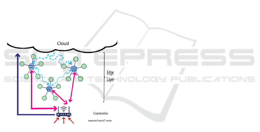
Request Processing. The communication between

IoT, edge and cloud nodes happens as follows. IoT

nodes can process requests locally or send them to

the controller for processing in the edge or the cloud.

Edge nodes can process incoming requests or, if un-

available, pass them to another edge node or the con-

troller. Cloud nodes process the allocated requests

and return the result to the IoT nodes, see Figure

1. The purpose of this study is to minimize total

execution time for IoT nodes in a proposed frame-

work based on edge computing.A controller decides

to which edge (or cloud) node to allocate a request.

The transfer time and the waiting (e.g., queueing

time) at the controller incur a delay.

Deﬁnition 1. A delay is the time spent by transfer-

ring a request to the next node and waiting there to be

processed. Thus, we typically have controller delays

, edge node delays D

and IoT node delays D

CLOSER 2020 - 10th International Conference on Cloud Computing and Services Science

330

The processing time is the time for execution at

a node, i.e., either a controller processing time P

an edge node processing time P

Deﬁnition 2. The response time R for an IoT node

is the time it takes to get a request processed, i.e., the

time between sending a request for processing until

receiving the result.

RT = D

+ P

+ D

+ P

+ D

This is also known as end-to-end latency in net-

worked environments.

The requests are generated by the IoT nodes with a

given deadline DL for processing and they are sent to

the controller for allocation of processing nodes. The

requests transferred from different IoT nodes get into

a queue until they ﬁnally get to the controller. The

controller will consider the total waiting time of all

edge nodes from their availability tables taking into

account the request deadline and will then allocate

the request to the best edge node with the lowest total

waiting time by applying PSO principles. The archi-

tectural framework of the edge-based system used in

this study is shown in Figure 1.

Figure 1: The IoT-Edge-Cloud architecture.

4.2 Controller Design

The controller is embedded as an orchestrator be-

tween the things layer and the edge. All requests from

the things layer will ﬁrst be transferred to the con-

troller and then sent to either the best edge node or

directly to the cloud. As said, the controller performs

the decision process based on the total waiting time

(delay) of the entire request in different edge nodes.

Upon receiving the new request, the controller deter-

mines the best node and allocates the request to that

node according to the deadline of the request and the

lowest total waiting time of all the edge nodes using

the particle optimization algorithm PSO. The status

of the selected node’s queue and it’s execution status

are updated in an availability table. If no appropriate

node is found in the edge layer for a received request,

the controller sends the request directly to the cloud

for processing as a backup.

Types of Cluster Coordination. Two types of in-

teraction for edge nodes can be implemented (Shin

and Chang, 1989): coordinated, in which some dedi-

cated nodes control the interactions of their surround-

ing nodes, fully distributed, in which each edge node

interacts with any other node. In the coordinated

method, the edge layer is divided into smaller clus-

ters, with a central coordinating node in each of these

clusters, which is directly interacting with the con-

troller and which controls the other nodes in its clus-

ter. This coordinator is aware of the queue status of

those nodes and stores all the information in the avail-

ability table. The central coordinating nodes are also

processing nodes which aside from their processing

responsibility, can manage the other nodes in their

clusters too. These central coordinators have 3 dif-

ferent connections, 2 direct connections and 1 pub-

lic connection. The central coordinators are directly

connected to their cluster’s nodes and the controller

and they communicate with other central coordina-

tors with public announces. When a request is sent

to the controller, the cluster coordinators announce

their best node in their area (personal best) publicly

and support the lead controller in determining the best

node in the layer (global best). This step is repre-

sented in Equation (6).

4.3 Optimization

In the third step, the PSO-based edge performance

optimization problem is deﬁned. In our method,

the optimization problem has one main objective and

one sub-objective so that the realization of the sub-

objective will lead to the fulﬁlling the main objective.

In the following, each of these goals will be deﬁned.

• Main objective: to minimize the total response

time R. In the proposed method, two elements,

the controller and the particle optimization algo-

rithm, have been used to accomplish this goal.

• Secondary objective: to reduce delay D. Delays in

each layer must be considered separately to calcu-

late the total delay.

We use (Yousefpour et al., 2017) to calculate delays.

Delay in Things Layer. Note that thing nodes can

both process requests themselves or send them to the

edge or cloud for processing. If an IoT node decides

to send their request to the edge or cloud for process,

the request will be sent to the controller ﬁrst. Con-

sidering the number of the IoT nodes and the num-

ber of the requests, the sent request will get into a

Particle Swarm Optimization for Performance Management in Multi-cluster IoT Edge Architectures

331

queue before reaching the controller and after reach-

ing the controller, the request should wait until the

controller ﬁnds the best edge node for allocation. In

other words, this is the delay before allocation.

Note, we adopt the notational settings as follows:

The subscript indexes i, j and k refer to processing

nodes at IoT, Edge and Cloud layer, respectively. The

superscripts I, E and C refer to source or destination

of transferred requests or responses at IoT, Edge or

Cloud level, respectively. For example, EC refers to

an edge-to-cloud transfer.

Deﬁnition 3. The delay in the IoT node i is repre-

sented by D

and is calculated as follows:

= P

× (A

) + P

× (X

i j

+ L

i j

) + P

× (X

+ H

+ X

)

(7)

• P

is the probability that the things node will pro-

cess the request itself in the things layer, P

the probability of sending the request to the edge

layer, and P

is the probability of sending the re-

quest directly to the cloud; with P

= 1.

• A

is the average processing delay of node i when

processing its request. X

i j

is the propagation de-

lay from object node i to node jj, Y

i j

is the sum

of all delays in linking from object node i to node

j. Likewise, X

delays propagation from object

node i to cloud k server and Y

is the sum of

all delays in sending a link from object node i

to cloud server k. X

and Y

are broadcast and

send delays from the k server to the node i.

• H is the average delay for processing a request

on the cloud server k, which includes the queue

waiting time on the cloud server k plus the request

processing time on the cloud server k.

There is no speciﬁc distribution for P

, P

and P

because their values will be deﬁned by separate ap-

plications based on service quality requirements and

rules. In other words, their values will be given as

input to this framework.

Delay in Edge Layer. We now deﬁne a recursive re-

lation for calculating L

i j

Deﬁnition 4. L

i j

is a delay for processing IoT node

i’s requests in the edge. After allocation, the re-

quest will be queued at the chosen edge node. This is

the delay after allocation. L

i j

is calculated as follows:

i j

= P

.(W

+ X

)

+ (1 + p

.[[1 − φ(x)][X

j j

+ L

i j

(x + 1)]

+ φ(x)[X

+ (H

+ X

]]

= best( j), k = h( j)

(8)

Here, W

refers to the mean waiting time at node j

and φ(x) is also a discharge function.

Delayed transmission from the cloud layer to the

object layer will be considered in L

i j

, as the request

edge later be unloaded to another node in the edge

layer. L

i j

is the processing delay of the node i request

in the edge layer or even the cloud layer, if it is un-

loaded from the edge node to the cloud server, so that

the node j edge be the ﬁrst node in the edge layer

to which the node request of object i is sent. All the

other variables already have been deﬁned.

4.4 PSO Algorithm Implementation

In the ﬁnal step, the performance optimization algo-

rithm is speciﬁed. The particle swarm optimization

algorithm is used to solve the optimization problem.

Our PSO algorithm consists of several steps, which

will be discussed now.

• Establish an Initial Population and Evaluate it.

The particle swarm optimization algorithm starts

with an initial random population matrix like

many evolutionary algorithms such as genetic al-

gorithms. This algorithm, unlike genetic algo-

rithms however, has no evolutionary operator such

as a mutant. Each element of the population is

called a node. In fact, the particle swarm opti-

mization algorithm consists of a ﬁnite number of

nodes that randomly take the initial value.

Here, the edge layer is divided into different clus-

ters and in each cluster consists of a central coor-

dinator node and its dependent nodes. For each

node, two states of location and velocity are de-

ﬁned, which are modeled with a location vector

and a velocity vector, respectively. These vectors

assist the controller in ﬁnding the best available

node. The location vector helps in ﬁnding the

position of the local best and the velocity vector

leads the controller towards the global best.

In Equations (7) and (8), all edge nodes j are pro-

cessing nodes. Selected nodes are also local co-

ordination nodes for the clusters. However, these

are not singled out in the equations since they also

have processing capacity.

• The Fitness Function. The ﬁtness function is

used for evaluating the initial population. Since

the problem is a two-objective optimization, both

goals must be considered in the ﬁtness function.

– The ﬁrst objective is to minimize the total re-

sponse time (latency) in the edge-based archi-

tecture indicated by RT .

To achieve the ﬁrst goal, we deﬁne a metric

called T

= P

+ D

that represents the total

CLOSER 2020 - 10th International Conference on Cloud Computing and Services Science

332

execution time of the request at the edge node,

which is the sum of the processing time P

of the request and the waiting time D

of the

request in the edge node’s queue. TimeFinal

(T F) is the maximum time T

that is allowed

for the execution at the edge node in other to

meet the required deadline DL with

T F = DL − (D

+ P

+ D

) (9)

i.e., Max(T

) = T F or T

∈ [0 . . . T F ].

– The second objective is to reduce the delay of

the edge-based architecture D.

The second goal relates to the sum of the delays

in the IoT layer and the delay in the edge layer:

D = D

+ D

(10)

Both goals are deﬁned as minimization. Ulti-

mately, ﬁtness is calculated as follows:

Fitness = T F + D (11)

• Determine the Best Personal Experience and the

Best Collective Experience. The nodes move in

the solution space at a dynamic rate based on the

experience of the node itself and the experience

of the neighbors in the cluster. Unlike other evo-

lutionary algorithms, particle swarm optimization

does not use smoothing operators (such as inter-

sections in the frog algorithm). Thus, the answers

remain in the search space to share their infor-

mation and guide the search to the best position

in the search space. So, here the coordinating

nodes search for the best experience within their

own and their neighbor’s domain. To update the

node’s velocity and position, ﬁrst the best position

of each node and then the best position among all

nodes in each step must be updated.

• Location and Velocity Updates. The dimension

of the problem space is equal to the number of

parameters in the function to optimize. The best

position of each node in the past and the best po-

sitions of all nodes are stored. Based on this, the

nodes decide how to move next. At each itera-

tion, all the nodes move in the next n-dimensional

space of the problem to ﬁnd the general optimum

point. The nodes update their velocities and their

position according to the best absolute and local

solutions. Here, the coordinating nodes read the

availability table of their cluster nodes and pub-

lish their best nodes to the controller. In this way,

they move towards the overall best node.

• Check the Termination Condition. Finally, the ter-

mination condition is checked. If this condition

is not met, we return to the stage of determining

the best personal experience and the best collec-

tive experience. There are several types of termi-

nation conditions:

– Achieve an acceptable level of response,

– Reach a speciﬁed number of repetitions/time,

– Reach a certain number of iterations or a time

speciﬁed without seeing an improvement,

– Check a certain number of responses.

Here, the termination condition is to achieve an

acceptable level of response.

Implementation. The proposed PSO Performance

Optimization is presented in Algorithm 1.

Algorithm 1: PSO-based Edge Performance.

1: function SCHEDULE(PSO,DAG)

2: Input: PSO and DAG characteristics

3: Output: Optimal Request Scheduling

4: Initial First Parameters

5: loop

6: Initial Population

7: Calculate Fitness

8: if Fitness < PBest then

9: PBest ← Fitness

10: GBest ← PBest

11: loop

12: Compute Velocity via Equation (1)

13: Compute Position via Equation (2)

14: Calculate Fitness via Equation (11)

15: if Fitness < PBest then

16: PBest ← Fitness

17: GBest ← PBest

18: Return: Optimal Schedule

5 EVALUATION

Our aim is to reduce the total response time – or end-

to-end latency. We chose a comparative experimental

approach to evaluate our solution.

The particle swarm optimization algorithm and a

so-called BAT algorithm (Yang, 2012) are used to es-

tablish the controller and compare. The BAT algo-

rithm was chosen due to its similarity to the particle

swarm optimization. Thus, it allows meaningful per-

formance comparisons. Furthermore, its wide-spread

use in different optimization situations make it a suit-

able benchmark. The BAT algorithm is an algorithm

inspired by the collective behavior of bats in the natu-

ral environment proposed in (Yang, 2012). This algo-

rithm is based on the use of bat reﬂection properties.

We used the MATLAB software to evaluate our

solution. The concepts presented earlier are fully

Particle Swarm Optimization for Performance Management in Multi-cluster IoT Edge Architectures

333

coded and implemented in MATLAB.

5.1 PSO & BAT Parameter Adjustment

In order to obtain meaningful results, this algorithm is

implemented with the dual-objective evaluation func-

tion according to Equation (11) with 200 iterations.

The initial parameters speciﬁed in this implementa-

tion are shown in Table 1. Using the values in Table 1

Table 1: Initial parameters - PSO Edge Optimization.

Parameters Values

Population number 50

Number of Repeats 200

Value w 1

Decrease coefﬁcient w 0.99

c1,c2,c3 2

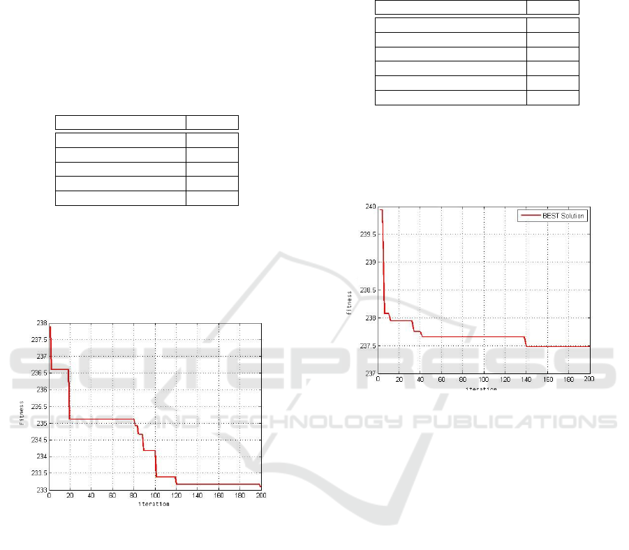
for initialization, the particle swarm optimization al-

gorithm is executed and the graph in Figure 2 shows

the result of the implementation of this algorithm in

terms of ﬁtness values for the respective iterations.

As shown in Figure 2, with the increase of iterations,

Figure 2: Fitness results for the PSO algorithm.

the results of the ﬁtness evaluation function for the

two objectives (runtime and delay) is reduced. Our

PSO performance optimization algorithm is a two-

objective algorithm that reduces execution time and

delay in execution of requests. The objective function

value in the implementation of the particle swarm op-

timization algorithm is approximately 233 as a bench-

mark for the BAT comparison. It should be noted that

due to the random structure of the evolutionary algo-

rithms, the results per run may be different from the

previous ones.

In order to comparatively evaluate our proposed

method, an evolutionary BAT algorithm has been im-

plemented in order to compare correctly with the

same conditions. Thus, the BAT algorithm has been

implemented with the same two-objective evaluation

function and with 200 iterations as the particle opti-

mization algorithm. The initial parameters speciﬁed

in this implementation are shown in Table 2. Using

Table 2: Initial parameters - BAT Optimization.

Parameters Values

Population number 50

Number of Repeats 200

Minimum frequency 0

Maximum frequency 100

Sound intensity coefﬁcient 0.1

Pulse rate coefﬁcient 0.1

the above values for the BAT strategy initialization,

the BAT algorithm is executed and the diagram in Fig-

ure 3 shows the result of the implementation of this al-

gorithm. In Figure 3, the motion diagram of the BAT

Figure 3: Fitness results for the BAT algorithm.

algorithm is shown. The conditions are the same for

both particle swarm and bat optimization algorithms

and the objective function in both algorithms has been

implemented and evaluated with respect to both run-

time and delay reduction. As can be seen, the BAT

algorithm has reached the target function of 237.5,

while in the particle swarm optimization algorithm

this value is 233. These results indicate that our algo-

rithm is better than the evolutionary BAT algorithm.

5.2 Scenario-based Comparison

In order to deepen the analysis, the proposed solution

was tested for 3 different scenarios: once with differ-

ent number of requests, once with different number of

edge layer nodes, once with identical parameters, but

in different iterations.

Scenario 1 – Request Variation. In the ﬁrst scenario,

a number of requests and nodes in the edge layer are

used to compare the results. In this scenario, we ﬁxed

the number of edge layers nodes and assumed vari-

able and incremental user requests. Table 3 shows the

details of this scenario conﬁguration.

Figure 4 shows the results of different user re-

CLOSER 2020 - 10th International Conference on Cloud Computing and Services Science

334

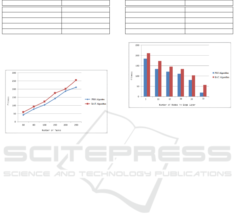
Table 3: The initial parameters in ﬁrst scenario.

Parameters Values

Number of user requests 30/60/100/150/200/250

Number of edge layer nodes 20

Processing power of each edge node 4 G Ram / 8 Mips Processor

Amount of time each user requests Randomized in range [1,20]

Amount of CPU per user request Random in the interval [2,8]

quests with 20 nodes in the edge layer. Here, the num-

ber of edge layer nodes is 20 and the number of user

requests are 30, 50, 100, 150, 200 and 250. Equation

(11) is used to calculate the ﬁtness function.

Figure 4: Result of 1st scenario: ﬁtness over no. of requests.

As can be seen in Figure 4, our PSO-based op-

timization algorithm produces far better results than

the BAT algorithm. As the number of requests in-

creases, the value of the target function (execution

time + delay time) increases. Increasing the number

of requests will increase the execution time, as well

as increase the execution time, as more nodes will be

involved. This increases the value of the target func-

tion, which is the sum of the execution time and de-

lay. In all cases, our PSO algorithm shows better re-

sults. Despite the increase in the objective function

value in both algorithms, the growth rate of the ob-

jective function value in the particle swarm optimiza-

tion algorithm is lower than the BAT algorithm, which

means that our algorithm outperforms BAT.

In order to compare under different conditions, the

next step is to increase the number of layer nodes in

order to observe the effect of this increase in a graph.

Scenario 2 – Edge Node Variation. In the second

scenario, unlike the previous scenario, now the num-

ber of requests is ﬁxed, but the number of edge layer

nodes is assumed to be variable. Increasing the num-

ber of nodes has been done as a trial-and-error exper-

iment and no special algorithm is used. Full details of

the second scenario are given in Table 4.

For this experiment, 100 input requests are consid-

ered. In this scenario, the number of user requests is

considered to be ﬁxed, but the number of edge layer

nodes is considered to be 5, 10, 15, 20, 30 and 50.

Table 4: The initial parameters in second scenario.

Parameters Values

Number of user requests 100

Number of edge layer nodes 5/10/15/20/30/50

Processing power of each edge node 4 G Ram / 8 Mips Processor

Amount of time each user requests Randomized in range [1,20]

Amount of CPU per user request Random in the interval [2,8]

Figure 5: 2nd scenario: ﬁtness over no. of requests.

Equation (11) is used to calculate the ﬁtness function.

By increasing the number of layer nodes in the

edge, the ﬁtness function decreases due to the pos-

sibility of executing requests on more nodes. The

higher the number of edge layer nodes, the more

likely it is that requests will be processed using nodes

whose latency is lower. In other words, with the in-

crease in the number of edge layer nodes the con-

troller’s options for allocating more requests are in-

creased and thus the chances of ﬁnding a suitable

node with low latency increases. As the conditions

change, the way in which requests are executed is also

varied, which reduces execution time. For the par-

ticle optimization algorithm, the greater the number

of edge layer nodes, the lower the objective function.

Furthermore, for PSO algorithm, the reduction of the

target function is much faster than the BAT algorithm,

which is evident in Figure 5. Each algorithm was run

multiple times to better compare the algorithms.

Scenario 3 – Iteration Variation. In the third sce-

nario, several iterations assume both the user requests

and the number of nodes in the edge layer ﬁxed. In

this scenario, each algorithm was run 5 times with the

same inputs and the results were obtained. It should

be noted that in this experiment, the number of re-

quests is 100 and the number of edge layer nodes is

50, which were constant at all 5 times. Equation (11)

is used to calculate the ﬁtness function. Table 5 shows

the full conﬁguration details of the third scenario. Ac-

cording to Figure 6, in different iterations we can see

different results despite not changing input values at

each iteration. There are no identiﬁable rules or ex-

planations detectable by analysing the algorithm out-

Particle Swarm Optimization for Performance Management in Multi-cluster IoT Edge Architectures

335

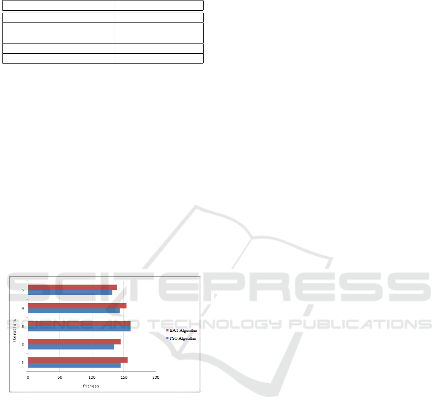
Table 5: The initial parameters in third scenario.

Parameters Values

Number of user requests 100

Number of Edge Layer Nodes 50

Processing power of each edge node 4 G Ram / 8 Mips Processor

Amount of time each user requests Randomized in range [1,20]

Amount of CPU per user request Random in the interval [2,8]

puts. For example, the value of the ﬁtness function

in the ﬁrst step with one iteration is less than that of

the BAT algorithm in PSO, and the value of this func-

tion in the second step with two iterations in both al-

gorithms decreased, while in the next step with three

iterations, the value is increased in both.

In general, it can be concluded that the node

swarm optimization algorithm in executing requests

using the dual-ﬁtness function (execution time + ex-

ecution delay) yields signiﬁcantly better results than

the evolutionary BAT algorithm. This is because in

most iterations, the objective function value in the

particle swarm optimization algorithm was lower than

for the BAT algorithm. A PSO feature is faster con-

vergence. In addition, the particle swarm optimiza-

tion algorithm yields overall good performance re-

sults that reduce orchestration and response time.

Figure 6: 2nd scenario: ﬁtness over number of requests.

6 CONCLUSIONS

Edge computing promises low latency due to local

processing. However, a closer look reveals distributed

and independently managed clusters of processing

edge nodes that need be considered in a performance-

oriented load allocation strategy. Furthermore, delays

occur as the result of transmission delays and waiting

times at orchestration and processing nodes.

In our performance optimization method, we used

an evolutionary algorithm based on particle swarm

optimization, adopted to the multi-cluster architecture

and focusing on delay and end-to-end latency reduc-

tion. We compared our solution with an evolution-

ary BAT algorithm, another method to optimize and

reduce the mean objective function (delay and ex-

ecution latency) of processing requests. Evolution-

ary algorithms are among the best optimization algo-

rithms, and the particle swarm optimization algorithm

we adopted here is less complex than some other evo-

lutionary algorithms. These advantages made the par-

ticle swarm optimization a suitable core of a method

for reducing the total execution time and delay.

As part of our future work, we plan to consider

other algorithm bases such as the ﬁreﬂy algorithm in-

stead of the node swarm optimization for edge perfor-

mance optimization. The ﬁreﬂy algorithm is a com-

mon algorithm in optimization problems that does not

have the limitations of genetic algorithms selecting

the required parameters, which is the most effective

choice for these operations. We could also consider

the ant colony algorithm or linear optimization in-

stead of PSO. The ant colony algorithm is very ef-

ﬁcient, often used in routing problems and the linear

optimization is a good method to achieve the best out-

come in a mathematical model whose requirements

are represented by linear relationships. Apart from the

algorithmic side, we also plan to reﬁne the model by

more precisely separating origins of propagation de-

lay in communication and buffering times. Also dif-

ferent coordination principles from fully centralised

to peer-to-peer management can be considered. And,

we aim to combine this with an auto-scaling con-

troller (Gand et al., 2020), which we implemented so

far only for a single cluster environment.

REFERENCES

Baktyan, A. A. and Zahary, A. T. (2018). A review on cloud

and fog computing integration for iot: Platforms per-

spective. EAI Transact on Internet of Things, 4(14).

Fang, D., Liu, X., Romdhani, I., Jamshidi, P. and Pahl, C.

(2016). An agility-oriented and fuzziness-embedded

semantic model for collaborative cloud service search,

retrieval and recommendation. In Future Generation

Computer Systems, 56, 11-26.

Gand, F., Fronza, I., Ioini, N. E., Barzegar, H. R., Azimi,

S., and Pahl, C. (2020). A fuzzy controller for self-

adaptive lightweight container orchestration. In Intl

Conf on Cloud Computing and Services Science.

Gand, F., Fronza, I., El Ioini, N., Barzegar, H. R. and Pahl,

C. (2020). Serverless Container Cluster Management

for Lightweight Edge Clouds. In Intl Conference on

Cloud Computing and Services Science CLOSER.

Gand, F., Fronza, I., El Ioini, N., Barzegar, H. R. and Pahl,

C. (2020). A Lightweight Virtualisation Platform for

Cooperative, Connected and Automated Mobility. In

6th Intl Conference on Vehicle Technology and Intelli-

gent Transport Systems (VEHITS).

CLOSER 2020 - 10th International Conference on Cloud Computing and Services Science

336

González, L. M. V. and Rodero-Merino, L. (2014). Finding

your way in the fog: Towards a comprehensive def-

inition of fog computing. Computer Communication

Review, 44(5):27–32.

Gu, L., Zeng, D., Guo, S., Barnawi, A., and Xiang, Y.

(2017). Cost efﬁcient resource management in fog

computing supported medical cyber-physical system.

Trans on Emerging Topics in Computing.

El Ioini, N., Pahl, C. and Helmer, S. (2018). A decision

framework for blockchain platforms for IoT and edge

computing. IoTBDS’18.

Jamshidi, P., Pahl, C., Chinenyeze, S. and Liu, X. (2015).

Cloud Migration Patterns: A Multi-cloud Service Ar-

chitecture Perspective. In Service-Oriented Comput-

ing - ICSOC 2014 Workshops. 6–19.

Jamshidi, P., Pahl, C. and Mendonca, N. C. (2016). Man-

aging uncertainty in autonomic cloud elasticity con-

trollers. IEEE Cloud Computing, 50-60.

Jamshidi, P., Pahl, C. and Mendonca, N. C. (2017). Pattern-

based multi-cloud architecture migration. Software:

Practice and Experience 47 (9), 1159-1184.

Mahmud, R., Srirama, S. N., Ramamohanarao, K., and

Buyya, R. (2019). Quality of experience (qoe)-aware

placement of applications in fog computing environ-

ments. J. Parallel Distrib. Comput., 132:190–203.

Manasrah, A. and Ali, H. (2018). Workﬂow scheduling

using hybrid ga-pso algorithm in cloud computing.

Wireless Comm and Mobile Comp, 2018:1–16.

Mendonca, N. C., Jamshidi, P., Garlan, D. and Pahl, C.

(2020). Developing Self-Adaptive Microservice Sys-

tems: Challenges and Directions. In IEEE Software.

Meng, H., Zhu, Y., and Deng, R. (2017). Optimal comput-

ing resource management based on utility maximiza-

tion in mobile crowdsourcing. Wireless Communica-

tions and Mobile Computing, 2017.

Minh, Q. T., Nguyen, D. T., Le, V. A., Nguyen, D. H., and

Pham, T. V. (2019). Task placement on fog computing

made efﬁcient for iot application provision. Wireless

Communications and Mobile Computing.

Omara, F. A. and Arafa, M. M. (2010). Genetic algorithms

for task scheduling problem. Journal of Parallel and

Distributed Computing, 70(1):13 – 22.

Pahl, C., Jamshidi, P., and Zimmermann, O. (2018). Archi-

tectural principles for cloud software. ACM Transac-

tions on Internet Technology (TOIT), 18(2):17.

Pahl, C., El Ioini, N., Helmer, S. and Lee, B. (2018). An ar-

chitecture pattern for trusted orchestration in IoT edge

clouds. Intl Conf Fog and Mobile Edge Computing.

Pahl, C., Fronza, I., El Ioini, N. and Barzegar, H. R. (2019).

A Review of Architectural Principles and Patterns for

Distributed Mobile Information Systems. In 14th Intl

Conf on Web Information Systems and Technologies.

Pahl, C., Jamshidi, P. and Zimmermann, O. (2020). Mi-

croservices and Containers. Software Engineering

SE’2020.

Rolim, C. O., Koch, F. L., Westphall, C. B., Werner, J.,

Fracalossi, A., and Salvador, G. S. (2010). A cloud

computing solution for patient’s data collection in

health care institutions. eTELEMED.

Saboori, A., Jiang, G., and Chen, H. (2008). Autotuning

conﬁgurations in distributed systems for performance

improvements using evolutionary strategies. In Intl

Conf on Distributed Computing Systems.

Samir, A. and Pahl, C. (2020). Detecting and Localizing

Anomalies in Container Clusters Using Markov Mod-

els. Electronics 9 (1), 64.

Sarkar, S., Chatterjee, S., and Misra, S. (2018). Assessment

of the suitability of fog computing in the context of

internet of things. Trans. Cloud Computing.

Scolati, R., Fronza, I., El Ioini, N., Samir, A. and Pahl,

C. (2019). A Containerized Big Data Streaming Ar-

chitecture for Edge Cloud Computing on Clustered

Single-Board Devices. International Conference on

Cloud Computing and Services Science.

Shin, K. G. and Chang, Y. (1989). Load sharing in dis-

tributed real-time systems with state-change broad-

casts. IEEE Trans. Computers, 38(8):1124–1142.

Tata, S., Jain, R., Ludwig, H., and Gopisetty, S. (2017).

Living in the cloud or on the edge: Opportunities and

challenges of iot application architecture. In Intl Conf

on Services Computing (SCC).

von Leon, D., Miori, L., Sanin, J., El Ioini, N., Helmer,

S. and Pahl, C. (2018). A Performance Exploration

of Architectural Options for a Middleware for Decen-

tralised Lightweight Edge Cloud Architectures. Intl

Conf Internet of Things, Big Data & Security.

von Leon, D., Miori, L., Sanin, J., El Ioini, N., Helmer, S.

and Pahl, C. (2019). A Lightweight Container Mid-

dleware for Edge Cloud Architectures. Fog and Edge

Computing: Principles and Paradigms, 145-170.

Wang, Z., Shi, B., and Zhao, E. (2001). Bandwidth-

delay-constrained least-cost multicast routing based

on heuristic genetic algorithm. Computer Communi-

cations, 24:685–692.

Wang, Z., Zhao, Z., Min, G., Huang, X., Ni, Q., and Wang,

R. (2018). User mobility aware task assignment for

mobile edge computing. Future Gen Comp Systems.

Yang, X.-S. (2012). Bat algorithm for multi-objective opti-

misation. arXiv preprint arXiv:1203.6571.

Yousefpour, A., Ishigaki, G., and Jue, J. P. (2017). Fog

computing: Towards minimizing delay in the internet

of things. In Intl Conf on Edge Computing EDGE’17.

Particle Swarm Optimization for Performance Management in Multi-cluster IoT Edge Architectures

337