Estimating Problem Instance Difﬁculty

Hermann Kaindl, Ralph Hoch and Roman Popp

Institute of Computer Technology, TU Wien, Austria

Keywords:

Case-based Reasoning, Similarity Metric, Heuristic Search, Admissible Heuristic, Problem Difﬁculty.

Abstract:

Even though for solving concrete problem instances, e.g., through case-based reasoning (CBR) or heuristic

search, estimating their difﬁculty really matters, there is not much theory available. In a prototypical real-

world application of CBR for reuse of hardware/software interfaces (HSIs) in automotive systems, where the

problem adaptation has been done through heuristic search, we have been facing this problem. Hence, this

work compares different approaches to estimating problem instance difﬁculty (similarity metrics, heuristic

functions). It also shows that even measuring problem instance difﬁculty depends on the ground truth available

and used. A few different approaches are investigated on how they statistically correlate. Overall, this paper

compares different approaches to both estimating and measuring problem instance difﬁculty with respect to

CBR and heuristic search. In addition to the given real-world domain, experiments were made using sliding-

tile puzzles. As a consequence, this paper points out that admissible heuristic functions h guiding search

(normally used for estimating minimal costs to a given goal state or condition) may be used for retrieving

cases for CBR as well.

Notation

s,t Start node and goal node, respectively

c(m, n) Cost of the direct arc from m to n

k(m, n) Cost of an optimal path from m to n

∗

(n) Cost of an optimal path from s to n

∗

(n) Cost of an optimal path from n to t

g(n), h(n) Estimates of g

∗

(n) and h

∗

(n), respectively

f (n) Static evaluation function: g(n) + h(n)

∗

Cost of an optimal path from s to t

N# Number of nodes generated

1 INTRODUCTION

There is a lot of theory on complexity classes of

problems, e.g., the famous issue of P vs. NP, but

not much on the difﬁculty of solving concrete prob-

lem instances of the same problem class (e.g., the

well-known Fifteen Puzzle, see http://kociemba.org/

themen/ﬁfteen/ﬁfteensolver.html). For solving con-

crete problem instances, e.g., through heuristic search

(Edelkamp and Schroedl, 2012; Pearl, 1984), how-

ever, estimating their difﬁculty really matters. Often,

this is done there through heuristic functions h(n),

which estimate the cost from this particular instance

n to a goal. In case-based reasoning (CBR) (see,

e.g., (Goel and Diaz-Agudo, 2017)), estimating the

effort for adapting some stored solution of a previ-

ously solved problem instance to a solution of a new

problem instance is often indirectly addressed by re-

trieving the nearest neighbor determined through sim-

ilarity metrics. The underlying assumption is that

the relative effort for solution adaptation of stored in-

stances (cases) correlates with the similarity of these

instances with the given problem instance.

In fact, there are two different views of problem

difﬁculty involved here:

• The cost of the solution, and

• The effort of ﬁnding a solution.

Depending on the view taken, C

∗

(the cost of an op-

timal path from the start node s to a goal node t) is

a good measure of problem difﬁculty in terms of the

cost of a solution (for its execution by a robot, for in-

stance), while the number of nodes generated and the

time needed for ﬁnding a solution are good measures

for the difﬁculty in terms of the effort for ﬁnding a so-

lution. (Korf et al., 2001) provide an excellent study

of the relation between the two for IDA* and opti-

mal solutions. For ﬁnding error-bounded solutions,

there is a trade-off, and ﬁnding any solution usually

requires much less effort, of course.

For both heuristic search and CBR, this paper

compares different approaches to estimating prob-

lem instance difﬁculty. Originally, the motivation

for this investigation came from a prototypical real-

world application of CBR, where the problem adap-

Kaindl, H., Hoch, R. and Popp, R.

Estimating Problem Instance Difﬁculty.

DOI: 10.5220/0009390003590369

In Proceedings of the 22nd International Conference on Enterprise Information Systems (ICEIS 2020) - Volume 1, pages 359-369

ISBN: 978-989-758-423-7

359

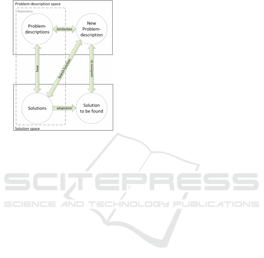
Figure 1: Terminology Clariﬁcation.

tation has been done through heuristic search, see

(Rathfux et al., 2019a; Rathfux et al., 2019b). More

speciﬁcally, this heuristic search uses A* (Hart et al.,

1968), so that the solutions have guaranteed minimal

cost (actually, a minimum number of steps), which

was desired in this domain. The overall theme of

this work was reusing hardware/software interfaces

(HSIs) in automotive systems. After having a stored

most similar one selected and retrieved, its conﬁg-

uration is transformed to another one that fulﬁls all

the new requirements. The number of transformation

steps is desired to be minimal in order to avoid hav-

ing to create new hardware. Since we deﬁned an ad-

missible heuristic h, A* guarantees optimal solutions.

An interesting question was then, whether to use this

heuristic h instead of similarity metrics for selecting a

stored HSI.

In order to avoid potential misunderstandings of

certain key notions (such as “solution”) in this combi-

nation of heuristic search and CBR, Figure 1 provides

an overview. It distinguishes a problem-description

space and a solution space. Each stored case in the

repository has a representation in both spaces. In the

problem-description space, the requirements on a new

HSI are speciﬁed, and in the solution space the inter-

nal conﬁguration of the HSI fulﬁlling them is stored.

Heuristic search is used here for ﬁnding a solution

in the sense of a sequence of transformations from a

given HSI to another one that fulﬁlls the requirements

(which deﬁne the goal conditions for the search). In

CBR, a major step is the selection of the “best” case

in the repository for adaptation of its stored solution

(here in the sense of a given HSI) to a solution of

the new case (an HSI fulﬁlling the new requirements).

While this selection is usually done through similar-

ity metrics, in the special case of automatic adaption

using heuristic search, there is the additional possibil-

ity to estimate the adaptation effort using its heuristic

function.

For studying different estimation techniques (in

the sense of heuristic functions and similarity metrics)

more generally, we also employed the well-known

Fifteen Puzzle. In contrast to the real-world domain,

it is widely known and was often used in the litera-

ture on heuristic search. All the results can be eas-

ily replicated publicly. This version of the sliding-

tile puzzle is only used here as a vehicle for compar-

ing such estimates (including simpler and less precise

ones) and not for presenting a new search algorithm

that would be faster than any other before (by using

the best heuristic estimate known), when the Twenty-

four Puzzle would have to be the choice today, such

as in (Bu and Korf, 2019).

Comparing different estimates needs to refer to

“real” problem instance difﬁculty, whatever this may

mean precisely. However, this raises yet another is-

sue, how that can be measured. For the Fifteen Puz-

zle, usually the instances are ordered according to the

lengths of their minimal solution paths C

∗

(due to unit

costs, the length is the same here as the cost of an

optimal path). But how well do they correlate with

the numbers of nodes explored by some algorithm for

solving them? And how do the numbers of nodes

explored by, e.g., A* correlate with those of IDA*

(Korf, 1985)? In addition, it makes a (theoretically

understood) difference of whether optimal solutions

are to be found, or solutions with a bounded error,

or just any solutions. For our experiment, we deal

here with ﬁnding optimal solutions through heuristic

search, since it provides a well-deﬁned case for com-

paring the search effort with estimates.

Hence, this paper actually compares different ap-

proaches to both estimating and measuring problem

(instance) difﬁculty with respect to CBR and heuris-

tic search. For estimating, we employ both various

similarity metrics and different h functions. For mea-

suring problem instance difﬁculty, we employ mini-

mum solution length (cost), the number of nodes gen-

erated for solving them by some algorithm, and two

new measures very recently deﬁned by us in (Rathfux

et al., 2019b).

The remainder of this paper is organized in the fol-

lowing manner. First, we present some background

material and discuss related work, in order to make

this paper self-contained. Then we explain several

approaches to measuring problem instance difﬁculty,

followed by explaining several approaches to estimat-

ICEIS 2020 - 22nd International Conference on Enterprise Information Systems

360

ing it. Based on all that, we present our experimental

results and interpret them. Finally, we provide a con-

clusion based on our experimental results.

2 BACKGROUND AND RELATED

WORK

2.1 CBR in a Nutshell

Case-based Reasoning (CBR) is an approach to solve

problem instances based on previously solved prob-

lem instances (Kolodner, 1993). It is assumed to

be closely related to the way a person solves prob-

lems: by recalling past experiences and applying that

knowledge to the new problem, or in other words,

mapping the new problem to previous experiences.

For the cognitive science foundations of CBR see

(Lopez de Mantaras et al., 2005).

The ﬁrst CBR systems have been developed in the

early 1980s and were based on the work of (Schank,

1983). Essentially, CBR is a cyclic process for solv-

ing problems (Aamodt and Plaza, 1994) and consists

of four major process steps. First, a ﬁtting problem

instance for a new problem instance is retrieved from

the repository. This step is typically performed us-

ing similarity metrics. Next, the solution of the re-

trieved problem instance is reused by adapting it to

the new problem instance. Note, that his step may be

supported by an automatic adaption of the given prob-

lem instance to the new one by using, e.g., heuristic

search. The resulting solution is then tested and, if

necessary, revised. Finally, the resulting solution is

stored, together with the new problem instance, in the

repository, i.e., the new knowledge is retained in the

repository.

CBR has been applied in a variety of domains,

see, e.g., (Burke et al., 2006; Bulitko et al., 2010;

Kaindl et al., 2010). Search techniques have been

used to help optimize a CBR system for predicting

software project effort in (Kirsopp et al., 2002). An

early combination of CBR with minimax search for

game-playing can be found in (Reiser and Kaindl,

1995).

2.2 Similarity Metrics

Similarity metrics (Cha, 2007) are used to determine

how similar two objects are to each other, e.g., in

CBR. It is an approach commonly used in informa-

tion retrieval systems, e.g., to compare text docu-

ments, or for clustering of data in data mining appli-

cations (Bandyopadhyay and Saha, 2012). For each

object, a similarity value can be calculated in relation

to another object, i.e., each pair of objects has a simi-

larity score assigned. Thus, attributes of objects need

to be quantiﬁed so that they can be used in similarity

metrics. Typically, similarity scores are normalized

values in the interval [0, 1], where 0 indicates no sim-

ilarity at all and 1 indicates maximum similarity. A

popular similarity metric, among others, is the Cosine

Similarity (Sohangir and Wang, 2017).

2.3 A* and IDA*

The traditional best-ﬁrst search algorithm A* (Hart

et al., 1968) maintains a list of so-called open nodes

that have been generated but not yet expanded, i.e.,

the frontier nodes. It always selects a node from this

list with minimum estimated cost, one of those it con-

siders “best”. This node is expanded by generating

all its successor nodes and removed from this list. A*

speciﬁcally estimates the cost of some node n with an

evaluation function of the form f (n) = g(n) + h(n),

where g(n) is the (sum) cost of a path found from s to

n, and h(n) is a heuristic estimate of the cost of reach-

ing a goal from n, i.e., the cost of an optimal path

from s to some goal t. If h(n) never overestimates this

cost for all nodes n (it is said to be admissible) and

if a solution exists, then A* is guaranteed to return an

optimal solution with minimum cost C

∗

(it is also said

to be admissible). Under certain conditions, A* is op-

timal over admissible unidirectional heuristic search

algorithms using the same information, in the sense

that it never expands more nodes than any of these

(Dechter and Pearl, 1985). The major limitation of

A* is its memory requirement, which is proportional

to the number of nodes stored and, therefore, in most

practical cases exponential.

IDA* (Korf, 1985) was designed to address this

memory problem, while using the same heuristic eval-

uation function f (n) as A*. IDA* performs iterations

of depth-ﬁrst searches. Consequently, it has linear-

space requirements only. IDA*’s depth-ﬁrst searches

are guided by a threshold that is initially set to the

estimated cost of s; the threshold for each succeed-

ing iteration is the minimum f -value that exceeded

the threshold on the previous iteration. While IDA*

shows its best performance on trees, one of its major

problems is that in its pure form it cannot utilize du-

plicate nodes in the sense of transpositions. A trans-

position arises, when several paths lead to the same

node, and such a search space is represented by a di-

rected acyclic graph (DAG). IDA* “treeiﬁes” DAGs,

and this disadvantage of IDA* relates to its advantage

of requiring only linear space.

In principle, we could have used for this research

Estimating Problem Instance Difﬁculty

361

other search algorithms as well, e.g., with limited

memory (Kaindl et al., 1995) or for bidirectional

search. (Kaindl and Kainz, 1997), but experiments

using A* and IDA* were sufﬁcient.

2.4 HSI Domain

We use the real-world domain of Electronic Control

Units (ECUs) and HSIs in automotive vehicles for

our experiment. In this domain, each ECU provides

an HSI through which external hardware components

can communicate with internal software functions.

The software of these ECUs runs on a microcontroller

with internal resources, and the external hardware

components require some of them for functioning as

needed. In addition, hardware components may be

placed on the ECU to pre-process signals from exter-

nal hardware, so that they can be mapped to or access

resources. The external hardware is connected to the

ECU via pins, and the ECU-pins are routed through

hardware components on the ECU to pins of the mi-

crocontroller (µC-pin). Each µC-pin is internally con-

nected to several resources, e.g., an Analog-Digital-

Converter (ADC). The hardware components together

with selected resources on connected µC-pins provide

a speciﬁc interface type on an ECU-Pin, which an ex-

ternal hardware can use. All the selected interface

types together specify the HSI.

External hardware requires certain functionality

on ECU-pins for its own functioning as needed.

Therefore, requirements are speciﬁed that an ECU

and its HSI have to fulﬁll. An ECU is only satisfac-

tory for the customer if all requirements of all exter-

nal hardware are met. To fulﬁll requirements, spe-

ciﬁc types of resources in the microcontroller (µC-

Resources) have to be made available to ECU-pins via

hardware components. The connections of ECU-pins

to hardware components and from hardware compo-

nents to µC-pins are ﬁxed. Each µC-pin is connected

to several µC-Resources, but only one of them can be

used at the same time. However, which µC-Resource

is selected on a speciﬁc ECU is variable and can be

conﬁgured. Hence, this variability provides options

to fulﬁll requirements. In essence, this variability de-

ﬁnes the search space for ﬁnding optimal solutions.

This domain knowledge is captured in the meta-

model published in our previous work (Rathfux et al.,

2019a), where also HSI problem instances and so-

lutions are included. We employ design-space ex-

ploration using the VIATRA2 tool (Hegedus et al.,

2011), which provides an infra-structure for heuris-

tic search based on model-transformations, which im-

plement activating or deactivating a connection to a

µC-Resource on the model, until all the goal condi-

tions are fulﬁlled as speciﬁed by the requirements.

VIATRA2 also provides an implementation of A*,

for which we deﬁned an admissible heuristic function

in (Rathfux et al., 2019b).

Note, that that the overhead of A* for maintaining

its priority queue does not matter in such a model-

driven implementation, since it can only visit about

1,000 nodes per second for our application on a state-

of-the-art laptop. In a very efﬁcient implementation

of the Fifteen Puzzle in C, A* can visit on the same

hardware three orders of magnitude more nodes per

second, and IDA* even four.

3 MEASURING AND

ESTIMATING PROBLEM

INSTANCE DIFFICULTY

We provide here the deﬁnitions of measures and esti-

mates used in our experiment. Two of them are actu-

ally hybrids in the sense that a measure is combined

with an estimate.

3.1 Measuring

For measuring the difﬁculty of some problem instance

in some domain (as compared to the difﬁculty of other

problem instances), the question arises, what “prob-

lem instance difﬁculty” really means. Another ques-

tion is what ground truth is available and used for

measuring it. Of course, all of these measures are only

available after the fact, so that estimating is necessary

in practice (see below). However, our experiment had

them available, of course. For getting a better theoret-

ical understanding, it is still useful to study relations

between measures and estimates, see also (Korf et al.,

2001) for the number of nodes explored by IDA* us-

ing a given heuristic h, based on knowledge about its

distribution over the problem space.

According to one view, the difﬁculty of a prob-

lem instance is the running time it takes to solve it

(and indirectly also the size of memory used). This

time is usually proportional to the number of nodes

explored for a given algorithm like IDA* (with only

linear memory requirements). This depends on the

algorithm used, however! In particular, this is differ-

ent for A*, even though IDA* is conceptually derived

from A*. However, the memory need of A* grows

with the number of nodes explored, and maintaining

the stored nodes for fast access incurs additional over-

head.

According to the other view, which is independent

from a speciﬁc algorithm, is C

∗

, the cost of an opti-

ICEIS 2020 - 22nd International Conference on Enterprise Information Systems

362

mal path from s to t (for unit costs, its length). The

assumption is that C

∗

of a given problem instance cor-

relates with the time it takes for solving it. How strong

is this correlation actually?

3.2 Estimating

For estimating problem instance difﬁculty, let us dis-

tinguish here admissible heuristics from similarity

metrics, where the former are employed for heuristic

search and the latter for CBR.

3.2.1 Admissible Heuristics

Such heuristics fully depend, of course, on the prob-

lem domain. For the real-world HSI domain, we

had to develop an admissible heuristic on our own

before, which is sketched in (Rathfux et al., 2019a)

and more formally deﬁned in (Rathfux et al., 2019b).

Let us denote it as h

HSI

here. Since we followed the

constraint relaxation meta-heuristic (given already in

(Pearl, 1984)) for its development, h

HSI

is actually

consistent, but this is only relevant for our purposes

here for implying admissibility of h

HSI

For the Fifteen Puzzle domain previously stud-

ied in-depth, all the heuristics we include in our ex-

periment of estimating problem instance difﬁculty

are well-known, published and their admissibility is

proven. In fact, already in (Pearl, 1984) the constraint

relaxation meta-heuristic was illustrated for two such

heuristic functions:

• h

T R

, simply counting the number of tiles that are

positioned “right”, i.e., in the position as deﬁned

by the target conﬁguration t,

• h

, the so-called Manhattan Distance heuristic.

Both of them obviously return estimated numbers of

steps that are at least needed to arrive at the target

node t. While h

T R

provides only very rough esti-

mates, h

is obviously more accurate. Both, how-

ever, cannot compare with speciﬁcally pre-compiled

pattern databases, see (Felner et al., 2004). Essen-

tially, these cache heuristic values from breadth-ﬁrst

searches from the target node t backwards. In con-

trast to computing heuristic values on demand like

, pattern databases are pre-computed for later use

in heuristic search for some given problem instance.

They may largely differ in their sizes, e.g., a static

5-5-5 partitioning version requires about 3MB, 6-6-3

partitioning about 33MB, and 7-8 partitioning more

than half a GB. The heuristic function using these

small, medium-sized and large versions are denoted

below as h

P555

, h

P663

and h

P78

, respectively.

3.2.2 Similarity Metrics

One possibility to calculate similarity metrics is using

vectors encoding information. We studied different

variations on how to create such vectors.

In the HSI domain, we used bit-vectors. A bit-

vector is a vector where each entry is either true (1)

or false (0). We constructed the vectors using the re-

quirements given for each pin. A vector has n × i en-

tries, where n is the number of ECU-Pins and i is the

number of interface types. Each entry in the vector

corresponds to interface type it on ECU-Pin p and is

1 if his particular interface type is required on this pin.

Using these vectors, the heuristic value for s

H BIT

can

be calculated by counting the entries that are the same

in both the original vector and the vector to be com-

pared to. s

RR BIT

is deﬁned analogously, but instead of

counting the matching entries the differing entries are

counted. Hence, this is actually a dissimilarity metric.

Additionally, we constructed vectors using the in-

terface types of requirements at each ECU-Pin. In

contrast to the vectors described above, we used the

interface types directly (as a string representation) in

the vector. Hence, these vectors have a maximum of

n entries, where n is the number of ECU-Pins. It

is a maximum of n, since we did not include ECU-

Pins without interface types. Using such vectors, we

deﬁned a similarity metric s

where we counted the

conformance of interface types on ECU-Pins of two

HSIs. To normalize these similarity values, they are

divided by the number of rows of the larger vector.

A more usual approach to calculating similarity

metrics is using Cosine similarity, which essentially

calculates the angle between two vectors. Two vec-

tors that have the same orientation have a similarity

score of 1, where two vectors that are orthogonal to

each other have a similarity score of 0. This similarity

metric is not dependent on the domain and, thus, we

employed it in the HSI as well as the Puzzle domain.

The calculation of the cosine similarity is shown in

Equation 1.

Cos

(s) = cos(θ) =

A · B

kAk · kBk

∑

i=1

· B

∑

i=1

∑

i=1

(1)

In the HSI domain, we deﬁned the cosine similar-

ity s

COS BIT

using the same bit-vectors as for s

H BIT

By including the interface types of each requirement,

we deﬁned two interface similarity metrics s

and

IT R

. These metrics construct their vectors based on

all available interface types and count their occur-

rences. In s

IT R

, we additionally took the requirements

into account.

Estimating Problem Instance Difﬁculty

363

For the puzzle domain, we deﬁned the cosine sim-

ilarity s

COS

as well. We used the values of the tiles

and their positions for the construction of the vector

and compared it with the vector of the goal state.

For deﬁning another metric s

(s), we used the

count of all tiles that are already positioned correctly,

i.e., are in the same position they have to be in the

target state t, and divideed it by the number of tiles,

making it normalized in the interval [0, 1]. This metric

is shown in Equation 2.

(s) =

∑

n=0

TilePosCorrect

(2)

The same metric can also be deﬁned using the heuris-

tic h

T R

from above as shown in Equation 3.

(s) =

(3)

This approach is the same as the one for the Russel-

Rao Dissimilarity s

, where the tiles that are not in

the right position are used for its calculation.

3.3 Hybrids of Measuring and

Estimating

Since “blind” algorithms like Dijkstra’s famous

shortest-path algorithm cannot solve “difﬁcult” prob-

lem instances, algorithms like A* and IDA* employ

heuristic estimates h and still guarantee that a solution

found is optimal, if h is admissible (see also above).

The time they take for that heavily depends on the

quality of h used (see, e.g., (Pearl, 1984)). Hence, we

found it interesting to combine h with a measure into

a hybrid, for getting yet another view.

In fact, (Korf et al., 2001) showed that the ef-

fect of a heuristic function is to reduce the effective

depth of search by a constant, relative to a brute-force

search, rather than reducing the effective branching

factor. And especially for distinguishing “easy” prob-

lems in the HSI domain from the others, d

abs

turned

out to be very useful in (Rathfux et al., 2019b):

abs

(s) = C

∗

− h(s) (4)

rel

(s) =

abs

(s)

∗

(5)

For using d

rel

before, however, we did not yet gain

any experience. Still, it provides yet another view,

since d

abs

is most likely not very useful when com-

paring solutions with a large difference in cost.

Below, we use these formulas in the category of

measures, since by including C

∗

they cannot be used

for estimating in the course of a search for a newly

given problem instance.

4 EXPERIMENT

The experiment is designed to explore how these dif-

ferent approaches to estimating problem instance dif-

ﬁculty relate to measuring problem instance difﬁculty,

where also for the latter different approaches are com-

pared as listed above. Results on this relationship are

presented both using Pearson correlation coefﬁcients,

and how many selection errors the different estimates

make, as counted with respect to the various measur-

ing approaches. All this has been done in two do-

mains, the proprietary HSIs and the widely known

Fifteen Puzzle.

4.1 Experiment Design

First, we created a repository of problem instances

for both domains by running A* and for the Fifteen

Puzzle also IDA*, and with a variety of admissible

heuristics to ﬁnd optimal solutions. We stored for

each problem instance the values C

∗

, d

abs

, d

rel

and N#

(the number of nodes generated by A* and IDA*, re-

spectively). Since d

abs

, d

rel

also depend on the heuris-

tic used, we stored these values for each of them, and

the values calculated by the various heuristic func-

tions separately as well. In addition, we calculated the

values of a variety of similarity metrics (as explained

above) and stored them.

For studying the correlation between the values

of heuristic functions, similarity metrics and the

different measures of the ground truth, we calculated

Pearson correlation coefﬁcients:

r =

∑

i=1

− ¯x) · (y

− ¯y)

∑

i=1

− ¯x)

∑

i=1

− ¯y)

(6)

If the absolute value of a correlation coefﬁcient is

higher than the absolute value of another one, the ﬁrst

one indicates a stronger relationship. In fact, we ac-

tually calculated these coefﬁcients between all these

values, since we were interested in the correlations

among the estimates and also among the measures as

well.

However, Pearson correlation coefﬁcients are de-

ﬁned for linear correlations. h-values as estimates of

∗

, however, are usually exponentially related to the

number of explored nodes in searches by A*, IDA*

and the like, for ﬁnding optimal solutions. That is

why we determine Pearson correlation coefﬁcients

between h-values and the logarithm of the number of

nodes.

In addition, for each Pearson correlation coefﬁ-

cient we determined its signiﬁcance as the probabil-

ity p that it could be the result of random ﬂuctuation.

ICEIS 2020 - 22nd International Conference on Enterprise Information Systems

364

All the calculations of Pearson correlation coefﬁcients

and their signiﬁcance were run using Matlab.

In addition, we were interested in the respective

numbers of selection errors that each of the estimates

would make when being used for selecting a case

from a case base. An error means to select a case that

is worse than another one with respect to the problem

instance difﬁculty. Since we have different measures

for that, we were interested in the numbers of errors

for each of them. However, executing an experiment

directly with a case base and then ﬁnding optimal so-

lutions for each of its cases stored and the given goal

(state or condition, respectively) would be very ex-

pensive.

Instead, we used the repository initially created as

follows. For each of its entries, we deﬁned all the tu-

ples (est, di f f ) where for each est through a heuris-

tic function or similarity metric, respectively, and for

each measure of problem instance difﬁculty di f f , one

of the latter is assigned to the former. For each tu-

ple, we calculated how many errors it induces. To

calculate these errors, we ordered all tuples by their

similarity or heuristic values, respectively, in a vector,

and then checked it against the vector of the corre-

sponding measure. The assumption is that a higher

similarity value or a lower heuristic value, respec-

tively, indicates a case with lower problem instance

difﬁculty than another case with lower similarity or

higher heuristic value, respectively. Hence, the order

deﬁned by the respective measure should be the same,

e.g., the number of nodes generated N#. Given that,

an error is deﬁned to occur for a given tuple, if the

orders in the corresponding vectors are different.

As an example, let us consider two entries (15, 4)

and (16, 3), which are ordered in the sequence <

(15, 4), (16, 3) > based on their estimate. Since the

second tuple (16, 3) has a higher estimate but lower

difﬁculty measure, e.g., C

∗

, than the previous one,

then it is counted as an error.

As some values of the tuples in a given vector may

have the same similarity or heuristic value, respec-

tively, we shufﬂed all tuples and then ordered them,

introducing a different order of tuples with the same

estimate each time. We ran these process 100 times

for each measure and calculated the mean and median

values of the numbers of errors.

Of course, we included for both domains prob-

lem instances with varying difﬁculty. The C

∗

values

varied from 3 to 17 for the HSI domain, and from

41 to 66 for the Fifteen Puzzle. Since N# depends

on the algorithm used, we attempted to perform the

searches with both A* and IDA*, in order to investi-

gate the correlation between their respective N# val-

ues. Unfortunately, using IDA* is infeasible for the

more difﬁcult HSI problem instances due to the very

high number of DAGs in this search space. (There are

known means to address this, but then it would be-

come some variant of IDA*.) For the Fifteen Puzzle,

it was possible to solve all the 100 random instances

listed in (Korf, 1985) running A* on a state-of-the-art

laptop with 32GB of memory.

More precisely, we executed the experiment runs

on a standard Windows laptop computer with an In-

tel Core i7-8750H Processor (9MB Cache, up to 4.1

GHz, 6 Cores). It has a DDR4-2666MHz memory of

32GB. The disk does not matter, since all the experi-

mental data were gathered using the internal memory

only.

4.2 Experimental Results

After having run the experiment as designed above for

both the HSI domain and the Fifteen Puzzle, we got

the results as presented below.

4.2.1 HSI Domain

In the HSI domain, we used more than 1,000 HSI

speciﬁcations for our experiment. These speciﬁca-

tions have been randomly adapted from ten base con-

ﬁgurations and are spread across three categories:

Base5, Base7 and Base9. These categories indicate

the number of requirements that are already conﬁg-

ured and fulﬁlled by the HSI.

Each of the 1,000 cases has between three and

seventeen randomly selected requirements. For each

of these cases, their h

HSI

and their similarity values

(using a variety of metrics as deﬁned above) were

calculated with regard to ﬁtting base models, e.g.,

models using the same ECU. An automatic adapta-

tion from each of the 1,000 HSI speciﬁcations to ones

that satisfy the new requirements (as goal speciﬁca-

tions) has been performed through heuristic search

using A

∗

with our admissible heuristic function h

HSI

This guarantees an optimal solution C

∗

each, i.e., one

with a minimal number of adaptation steps.

For these data, all correlation coefﬁcients between

the measures of the ground truth and the heuris-

tic functions and similarity metrics, respectively, are

given in Table 1. All the data in this table are highly

statistically signiﬁcant with p < 0.01. A higher (ab-

solute) value indicates a stronger correlation with C

∗

and thus a better estimate. Some of these correlation

coefﬁcients are extremely high, such as the one be-

tween h

HSI

and C

∗

. That is, this heuristic function

is very good at estimating the number of steps mini-

mally required for solution adaptation. The reason is

that the vast majority of problem instances is “easy”

in the sense that they require no reconﬁgurations, and

Estimating Problem Instance Difﬁculty

365

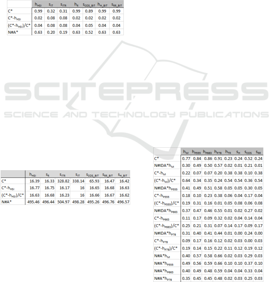
only a few problem instances actually require a few

reconﬁgurations, see (Rathfux et al., 2019b). Apart

from that, h

HSI

captures the knowledge for estimation

very well. It is actually because of this distribution

of problem instances that also some of the similar-

ity metrics correlate with C

∗

so strongly. The differ-

ence in the knowledge involved only matters for very

few problem instances here. For the absolute and the

relative error measures of the ground truth, however,

the correlation is very weak. The reason is that both

abs

= d

rel

= 0 for the majority of problem instances

here.

Table 1: Correlation coefﬁcients — HSI.

Even for the numbers of nodes generated by A*, more

precisely ln(N#A)*, the correlations with some of the

estimates are fairly high. For the given problem in-

stances, where only a few problem instances actually

require a few reconﬁgurations, these numbers can be

predicted well.

We also calculated the numbers of errors for the

heuristic function and each similarity metric. Table 2

shows the numbers of selection errors in the HSI do-

main. (More precisely these are the mean values as

explained above, and we omit the median values since

they are consistent with the mean values, i.e., outliers

do not play a role here.) In fact, the numbers of er-

rors of predicting N#A* are very high. The selection

results of predicting the other measures of the ground

truth are much better.

Table 2: Numbers of selection errors — HSI.

4.2.2 Fifteen Puzzle

As indicated above, we ran the set of 100 random Fif-

teen Puzzle instances published in (Korf, 1985) for

gathering their data on the different heuristics h

T R

, h

P555

, h

P663

and h

P78

, as well as the C

∗

, d

abs

and

rel

data (for the latter with all these heuristics). Since

both IDA* and A* were able to solve all those in-

stances even when using h

(but not with h

T R

), we

were also able to get the data on N#IDA* and N#A*,

more precisely the various numbers when using the

different heuristic functions (except h

T R

For these data, all correlation coefﬁcients between

the measures of the ground truth and the heuris-

tic functions and similarity metrics, respectively, are

given in Table 3. Note again, that we determined Pear-

son correlation coefﬁcients between each h-value and

the logarithm of the number of nodes. As a base, we

took the value 2.1304 from (Korf et al., 2001), since

it was determined there as the asymptotic branching

factor for the Fifteen Puzzle. Most of the data in this

table are highly statistically signiﬁcant with p < 0.01,

while especially those related to N#IDA* are only sta-

tistically signiﬁcant with p < 0.05, which is due to

the ﬂuctuation of the N#IDA* data. For the heuristic

functions used here, their respective domain knowl-

edge involved and their corresponding accuracy are

known. In fact, it is exactly reﬂected here in their

correlation with C

∗

. Estimates with more knowledge

correlate more strongly with C

∗

than the ones with

less knowledge. The similarity metric corresponding

to h

T R

in this regard, Hamming, has more or less the

same correlation coefﬁcient. In contrast, Cosine cor-

responds much better with C

∗

than Hamming. Still, its

(absolute) correlation coefﬁcient is much lower than

the ones of the heuristic functions incorporating more

domain knowledge. For the absolute and the relative

error measures of the ground truth, however, this pat-

tern is less clearly pronounced. d

abs

is very hard to

estimate for similarity metrics, which makes sense,

since a heuristic function is actually part of its calcu-

lation. However, also for heuristic functions estimat-

ing d

abs

is difﬁcult. The same applies to d

rel

Table 3: Correlation coefﬁcients — Fifteen Puzzle.

ICEIS 2020 - 22nd International Conference on Enterprise Information Systems

366

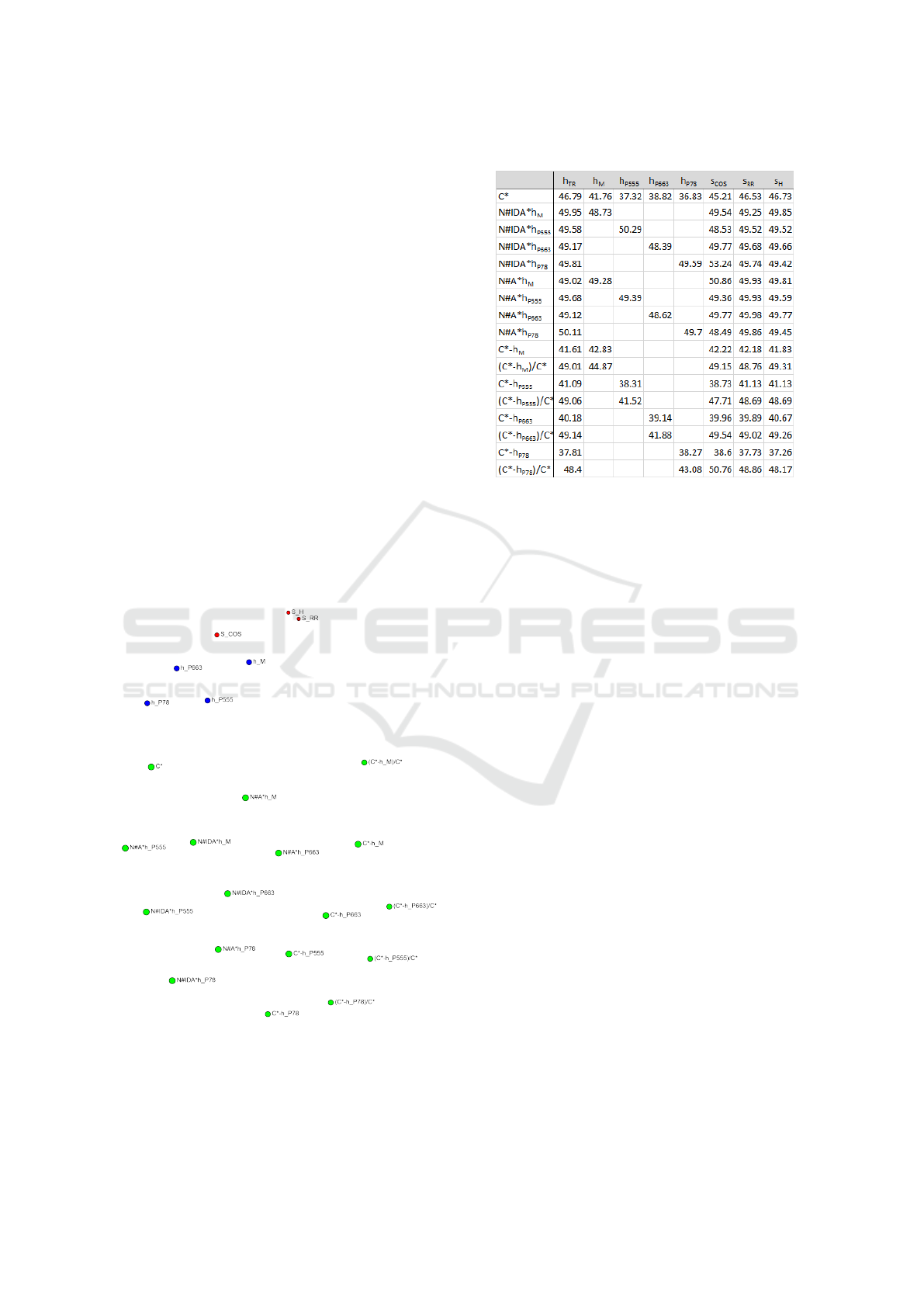
For the numbers of nodes generated by IDA* and

A*, respectively, more precisely their logarithm, the

correlations are lower than in the HSI domain. This

can be explained by the fact that the problem in-

stances in the HSI domain are much less difﬁcult,

both with respect to their solutions lengths and the

effort to determine optimal solutions (in terms of the

numbers of nodes explored). In addition, IDA* shows

stronger ﬂuctuations of these numbers than A*, when

both use the same admissible heuristic. This can also

be seen in Figure 2 (generated by a clustering algo-

rithm), where all the correlations are visualized as dis-

tances between nodes. If the distance between two

nodes is small then this indicates a strong correlation

and vice versa a larger distance indicates a weak cor-

relation. The distances in the picture between C

∗

and

the data points corresponding to the numbers of nodes

generated are not smaller than those between C

∗

and

most of the heuristic functions. The distance from C

∗

to the cluster of similarity metrics, however, is clearly

larger, and this corresponds well with the observation

made above, of course. In fact, all the heuristic func-

tions attempt to estimate C

∗

somehow, especially the

ones based on pattern databases and to a lesser extent

Figure 2: Two-dimensional clustering of correlations —

Fifteen Puzzle.

Overall, Figure 2 actually illustrates clusters. There

are two distinct clusters among the ground truth val-

ues. The ﬁrst one contains all N# values. Although

Table 4: Numbers of selection errors — Fifteen Puzzle.

these values vary strongly in the number of nodes,

they correlate well with each other. The second clus-

ter contains the variations of d

rel

and d

abs

. They do

not correlate well with estimating functions, but with

each other.

Finally, we also checked the number of errors dur-

ing selection, see Table 4. The somewhat surprising

result is, that a higher correlation coefﬁcient does not

necessarily carry over to a reduction of the number of

errors. As pointed out above, N# are hard to estimate

and even higher correlation coefﬁcients do not yield

lower error values when selecting. The best selections

results are accomplished in terms of C

∗

. In this case, a

higher correlation coefﬁcient also means fewer errors

during selection. Also, heuristics with more knowl-

edge provide better results, and the heuristic functions

lead to fewer selection errors than the similarity met-

rics in this regard.

5 CONCLUSION

In CBR, an underlying assumption is that the rela-

tive effort for solution adaptation of stored instances

(cases) correlates with the similarity of these in-

stances with the given problem instance. In our pro-

totypical real-world HSI application, heuristic search

is used for automatic solution adaptation. Hence,

we conjectured that admissible heuristic functions h

guiding search (normally used for estimating minimal

costs to a given goal state or condition) may be used

for retrieving cases for CBR as well. As a result of our

experiment, we actually conclude that the numbers of

selection errors can be reduced with regard to the opti-

mal solution length by using such heuristic functions,

Estimating Problem Instance Difﬁculty

367

if they have more knowledge incorporated than the

similarity metrics, and if the problem instances are

difﬁcult (as shown for the Fifteen Puzzle instances).

ACKNOWLEDGMENTS

The InteReUse project (No. 855399) has been funded

by the Austrian Federal Ministry of Transport, In-

novation and Technology (BMVIT) under the pro-

gram “ICT of the Future” between September 2016

and August 2019. More information can be found at

https://iktderzukunft.at/en/.

The VIATRA team provided us with their VIA-

TRA2 tool. Our implementations of Fifteen Puzzle

are based on the very efﬁcient C code of IDA* and

A* made available by Richard Korf and an efﬁcient

hashing schema by Jonathan Shaeffer. Ariel Felner

and Shahaf Shperberg provided us with hints about

the availability of code for the Fifteen Puzzle pattern

databases.

Last but not least, Alexander Seiler and Lukas

Schr

oer helped us with getting all the C code running

under Windows for our Fifteen Puzzle experiment.

REFERENCES

Aamodt, A. and Plaza, E. (1994). Case-based Reasoning:

Foundational Issues, Methodological Variations, and

System Approaches. AI Commun., 7(1):39–59.

Bandyopadhyay, S. and Saha, S. (2012). Unsuper-

vised Classiﬁcation: Similarity Measures, Classi-

cal and Metaheuristic Approaches, and Applications.

Springer Publishing Company, Incorporated.

Bu, Z. and Korf, R. E. (2019). A*+IDA*: A simple hy-

brid search algorithm. In Proceedings of the Twenty-

Eighth International Joint Conference on Artiﬁcial In-

telligence, IJCAI-19, pages 1206–1212. International

Joint Conferences on Artiﬁcial Intelligence Organiza-

tion.

Bulitko, V., Bj

ornsson, Y., and Lawrence, R. (2010). Case-

based subgoaling in real-time heuristic search for

video game pathﬁnding. J. Artif. Int. Res., 39(1):269–

300.

Burke, E. K., Petrovic, S., and Qu, R. (2006). Case-based

heuristic selection for timetabling problems. Journal

of Scheduling, 9(2):115–132.

Cha, S.-H. (2007). Comprehensive Survey on Dis-

tance/Similarity Measures between Probability Den-

sity Functions. International Journal of Mathematical

Models and Methods in Applied Sciences, 1(4):300–

307.

Dechter, R. and Pearl, J. (1985). Generalized best-

ﬁrst strategies and the optimality of a*. J. ACM,

32(3):505–536.

Edelkamp, S. and Schroedl, S. (2012). Heuristic

Search: Theory and Applications. Morgan Kaufmann,

Waltham, MA.

Felner, A., Korf, R. E., and Hanan, S. (2004). Additive pat-

tern database heuristics. J. Artif. Int. Res., 22(1):279–

318.

Goel, A. K. and Diaz-Agudo, B. (2017). What’s hot in case-

based reasoning. In Proc. Thirty-First AAAI Confer-

ence on Artiﬁcial Intelligence (AAAI-17), pages 5067–

5069, Menlo Park, CA. AAAI Press / The MIT Press.

Hart, P., Nilsson, N., and Raphael, B. (1968). A formal

basis for the heuristic determination of minimum cost

paths. IEEE Transactions on Systems Science and Cy-

bernetics (SSC), SSC-4(2):100–107.

Hegedus, A., Horvath, A., Rath, I., and Varro, D.

(2011). A Model-driven Framework for Guided De-

sign Space Exploration. In Proceedings of the 2011

26th IEEE/ACM International Conference on Auto-

mated Software Engineering, ASE ’11, pages 173–

182, Washington, DC, USA. IEEE Computer Society.

Kaindl, H. and Kainz, G. (1997). Bidirectional heuristic

search reconsidered. Journal of Artiﬁcial Intelligence

Research (JAIR), 7:283–317.

Kaindl, H., Kainz, G., Leeb, A., and Smetana, H. (1995).

How to use limited memory in heuristic search. In

Proc. Fourteenth International Joint Conference on

Artiﬁcial Intelligence (IJCAI-95), pages 236–242. San

Francisco, CA: Morgan Kaufmann Publishers.

Kaindl, H., Smialek, M., and Nowakowski, W. (2010).

Case-based reuse with partial requirements speci-

ﬁcations. In Proceedings of the 18th IEEE In-

ternational Requirements Engineering Conference

(RE’10), pages 399–400.

Kirsopp, C., Shepperd, M., and Hart, J. (2002). Search

heuristics, case-based reasoning and software project

effort prediction. In Proceedings of the 4th Annual

Conference on Genetic and Evolutionary Computa-

tion, GECCO’02, pages 1367–1374, San Francisco,

CA, USA. Morgan Kaufmann Publishers Inc.

Kolodner, J. (1993). Case-Based Reasoning. Morgan Kauf-

mann Publishers Inc., San Francisco, CA, USA.

Korf, R. (1985). Depth-ﬁrst iterative deepening: An op-

timal admissible tree search. Artiﬁcial Intelligence,

27(1):97–109.

Korf, R. E., Reid, M., and Edelkamp, S. (2001). Time

complexity of iterative-deepening-A*. Artiﬁcial In-

telligence, 129(1):199 – 218.

Lopez de Mantaras, R., McSherry, D., Bridge, D., Leake,

D., Smyth, B., Craw, S., Faltings, B., Maher, M. L.,

Cox, M. T., Forbus, K., and et al. (2005). Retrieval,

reuse, revision and retention in case-based reasoning.

The Knowledge Engineering Review, 20(3):215–240.

Pearl, J. (1984). Heuristics: Intelligent Search Strate-

gies for Computer Problem Solving. Addison-Wesley,

Reading, MA.

Rathfux, T., Kaindl, H., Hoch, R., and Lukasch, F. (2019a).

An Experimental Evaluation of Design Space Explo-

ration of Hardware/Software Interfaces. In Proceed-

ings of the 14th International Conference on Evalu-

ation of Novel Approaches to Software Engineering,

ENASE 2019, pages 289–296. INSTICC, SciTePress.

Rathfux, T., Kaindl, H., Hoch, R., and Lukasch, F. (2019b).

Efﬁciently ﬁnding optimal solutions to easy problems

ICEIS 2020 - 22nd International Conference on Enterprise Information Systems

368

in design space exploration: A* tie-breaking. In van

Sinderen, M. and Maciaszek, L. A., editors, Proceed-

ings of the 14th International Conference on Software

Technologies, ICSOFT 2019, Prague, Czech Republic,

July 26-28, 2019., pages 595–604. SciTePress.

Reiser, C. and Kaindl, H. (1995). Case-based reasoning for

multi-step problems and its integration with heuristic

search. In Haton, J.-P., Keane, M., and Manago, M.,

editors, Advances in Case-Based Reasoning, pages

113–125, Berlin, Heidelberg. Springer Berlin Heidel-

berg.

Schank, R. C. (1983). Dynamic Memory: A Theory of

Reminding and Learning in Computers and People.

Cambridge University Press, New York, NY, USA.

Sohangir, S. and Wang, D. (2017). Improved sqrt-cosine

similarity measurement. Journal of Big Data, 4(1):25.

Estimating Problem Instance Difﬁculty

369