Efﬁcient Representation of Very Large Linked Datasets as Graphs

Maria Krommyda, Verena Kantere and Yannis Vassiliou

School of Electrical and Computer Engineering, National Technical University of Athens, Athens, Greece

Keywords:

Big Data Exploration, Linked Datasets, Graphical Representation.

Abstract:

Large linked datasets are nowadays available on many scientiﬁc topics of interest and offer invaluable knowl-

edge. These datasets are of interest to a wide audience, people with limited or no knowledge about the

Semantic Web, that want to explore and analyse this information in a user-friendly way. Aiming to support

such usage, systems have been developed that support such exploration they impose however many limitations

as they provide to users access to a limited part of the input dataset either by aggregating information or by

exploiting data formats, such as hierarchies. As more linked datasets are becoming available and more people

are interested to explore them, it is imperative to provide an user-friendly way to access and explore diverse

and very large datasets in an intuitive way, as graphs. We present here an off-line pre-processing technique,

divided in three phases, that can transform any linked dataset, independently of size and characteristics to one

continuous graph in the two-dimensional space. We store the spatial information of the graph, add the needed

indices and provide the graphical information through a dedicated API to support the exploration of the infor-

mation. Finally, we conduct an experimental analysis to show that our technique can process and represent as

one continuous graph large and diverse datasets.

1 INTRODUCTION

The establishment of the RDF data model has made

available many large and diverse linked datasets from

a wide range of scientiﬁc areas

. Exploring and

querying these datasets as published, though, requires

extensive knowledge of the semantic web and expen-

sive infrastructure. As a result these datasets are inac-

cessible to a wider audience.

In order to alleviate this barrier, linked datasets

should be represented using a graph model, where

each entity is presented as a distinct object, and the in-

formation is explorable through multiple ﬁltering cri-

teria. In order to implement a user-friendly system,

a technique should be developed that will meet some

important challenges. To begin with, the technique

should be able to handle a wide range of datasets that

differ in characteristics

. Available datasets may have

from a few thousands to millions of elements, they

may also be incomplete, have no semantic annotations

or not follow any data model or hierarchy

In addition, the technique should provide an easy

https://lod-cloud.net/

https://www.w3.org/wiki/TaskForces/Community

Projects/LinkingOpenData/DataSets/Statistics

https://datahub.io/collections/linked-open-data

and user-friendly way to support the exploration of

the information. As an example, entities should be

distinct object and connections between them clearly

deﬁned, the complete dataset should be available and

the graph topology should be consistent to allow the

user to understand where the information is located.

The relevant but also the absolute position in the two-

dimensional space of the data objects should remain

the same regardless of the user actions. Furthermore,

plenty of functionalities should be available for the

exploration of the information. Keyword search, path

exploration, neighbour information, ﬁltering and ag-

gregation, should be available in a user-friendly way

without requiring knowledge of querying or program-

ming languages from the user. Last but not least, the

information should be available for multiple users si-

multaneously through commodity hardware such as

laptops and tablets. Processing that requires expen-

sive infrastructure should be handled by the server

side of the system and not by the devices of the users.

An overview of the techniques and systems that

have been developed to address some of these chal-

lenges is presented here.

An initial approach to the problem of the explo-

ration of large linked datasets focused on generic vi-

sualization systems. These systems aim to extract

the information of linked, semantically annotated,

106

Krommyda, M., Kantere, V. and Vassiliou, Y.

Efﬁcient Representation of Very Large Linked Datasets as Graphs.

DOI: 10.5220/0009389001060115

In Proceedings of the 22nd International Conference on Enterprise Information Systems (ICEIS 2020) - Volume 1, pages 106-115

ISBN: 978-989-758-423-7

datasets and present it through generic visualization

options. These visualization options are limited to

charts, such as column, line, pie, bar, scatter and

radar, that present the information in a summarized

way. Some systems (Voigt et al., 2012; Schlegel et al.,

2014) allow the dynamic choice of such visualization

types based on the user selection. The user can select

what information is of interest and the visualization

type to present it. Other systems (Brunetti et al., 2012;

ımek et al., 2013; Atemezing and Troncy, 2014)

utilize strict semantic rules and restrict the users to

predeﬁned types of visualizations.

These systems handle data ﬁtting speciﬁc crite-

ria regarding their structure and semantic information,

and present the information summarized in restrictive

forms. These approaches can give a general overview

of the information but cannot support the graphical

representation of the information. In addition, such

systems cannot handle datasets that are incomplete or

lack semantic annotations.

A large number of systems visualize linked

datasets adopting a graph-based approach (Mazumdar

et al., 2015). Some of these techniques (Abello et al.,

2006; Auber, 2004; Jr. et al., 2006) present small ﬁl-

tered or aggregated graphs of the input dataset based

on hierarchical data models. These systems use ag-

gregation and ﬁltering techniques to limit the size of

the represented graph and allow navigation only along

the hierarchy, making information inaccessible from

nodes at the same hierarchy level. While the naviga-

tion of highly aggregated data might help initially the

user to better understand the structure of the informa-

tion, at a deeper exploration of the dataset the loss of

information might be proven hindering to the useful-

ness of the representation.

The techniques discussed above meet only a sub-

set of the challenges. However, for many use cases,

such as road maps, communication networks and

blockchain transactions, it is of utmost importance to

meet all the challenges and not a subset of them.

Motivating Example. One of the most characteris-

tic examples of scientiﬁc data analysis that requires

a system that conforms to all the identiﬁed chal-

lenges, is the study and analysis of biological struc-

tures. Structural biology is a branch of molecular bi-

ology concerned with the molecular structure of bi-

ological macromolecules such as proteins, made up

of amino acids, how they acquire the structures they

have, and how alterations in their structures affect

their function. This subject is of great interest to bi-

ologists because macromolecules carry out most of

the functions of cells, and it is only by coiling into

speciﬁc structures that they are able to perform these

functions. The Protein Data Bank

is an archive

with information about the shapes of proteins, nucleic

acids, and complex assemblies. Most of the datasets

published there follow the Systems Biology Markup

Language

aiming to ensure model interoperability

and semantically correct information. As an example

we take the human cap-dependent 48S pre-initiation

complex

which represents 47 unique protein chains

with 116774 atom count.

Access to the Complete Information. Scientist aim-

ing to study and analyse this protein complex need to

have access to the complete information in a way that

will respect the initial spatial relations, without caus-

ing any alterations to connections between molecules.

Systems that use aggregation or summarization tech-

niques cannot be used for this analysis as they alter the

initial connections between atoms. Techniques that

exclude part of the input dataset if it does not follow

pre-deﬁned data formats cannot be used either, as pro-

tein chains are not expected to fully comply with spe-

ciﬁc data formats and atoms that deviate from them

contain important information which should be avail-

able to the user. Systems that ﬁlter the input dataset

based on speciﬁc characteristics cannot support the

exploration of protein complexes as their analysis is

mostly based on low level connections.

Combination of Multiple Datasets. In addition, scien-

tists need to study the complete biological structures,

so the system should be able to combine multiple pro-

tein chains and complexes. As an example, the human

cap-dependent 48S pre-initiation protein complex has

a relatively small number of atoms as it contains only

47 protein chains. Such complexes, however, are

combined or expanded with additional protein chains

for analysis purposes. The system should be able to

incorporate any additional information and offer to

the user exploration and ﬁltering services without any

limit to the size of the input dataset. Such dynamic

changes in the volume and content of the input dataset

is a challenge for all of the available systems. These

systems are based on complex pre-processing tech-

niques that aim to identify speciﬁc data models that

conform with the input dataset or perform a semantic

analysis and categorization. Due to their complexity,

such techniques fail to combine more than one dataset

or adapt to a large and complex one.

Multiple Filtering Criteria. Users interested in such

complex datasets also have high demands regarding

different and customizable ﬁltering functions that can

be used simultaneously. Popular queries during such

data analysis include: “isolate speciﬁc molecules” ,

https://www.rcsb.org/

http://semanticsbml.org/semanticSBML/simple/index

http://www.rcsb.org/structure/6FEC

Efﬁcient Representation of Very Large Linked Datasets as Graphs

107

“isolate one or more types of connections based on

their semantic annotations” , “identify the most/least

connected molecules” , “locate connections between

two molecules” , “ﬁnd if two or more molecules are

independent to one other” and “identify speciﬁc con-

nections in parts of the biological structure that is re-

sponsible for a speciﬁc function”.

The system should offer such exploration queries

though a user-friendly interface, without asking the

user to write queries over the data. Depending on the

way the information is processed, however, systems

may not be able to offer such exploration queries.

Systems that aggregate the input dataset cannot offer

details for one molecule. Systems that present data

based on hierarchy levels or through semantic criteria

cannot present the connections between two or more

molecules or isolate types of connections that are of

interest.

Path Exploration. Finally, given the importance

of the connections between molecules it is crucial

to identify all the neighbors of a molecule or follow

paths of interest. All of the available systems, allow

either the exploration of the outgoing neighbors of

a node or the exploration of nodes along the hierar-

chy levels of the data model. Therefore, the system

does not allow the user to intuitively explore the in-

formation associated with a node. For datasets such

as the human cap-dependent 48S pre-initiation pro-

tein complex, users are very interested in locating all

the neighbors of a molecule, either incoming or out-

going, as these connections are valuable to the protein

structure analysis.

Contribution. We present here an off-line pre-

processing technique that enables the Efﬁcient Rep-

resentation of Very Large Linked Datasets as Graphs.

Our technique has been carefully designed to alleviate

the restrictions of the above-mentioned approaches on

the input datasets, regarding accompanying metadata

related to the model, full or partial semantic anno-

tation, hierarchical structure, data completeness and

size limitation. It also meets the challenges of scal-

ability, consistent visualization and data exploration

through different ﬁltering functions. The proposed

technique is split into three phases, designed to trans-

form any input dataset, such as highly connected, in-

complete or lacking semantic annotations, into one

continuous graph on the two-dimensional space.

• Pre-processing Technique.

Initially, the input

dataset is split into smaller parts, the number and

size of which is determined by the dataset size

and connectivity degree. Next, each part of the

input dataset is graphically represented as an in-

dependent sub-graph. Finally, the sub-graphs are

merged into one continuous graph, using a suit-

able cost function that ensures small navigation

paths and consistent exploration for millions of

nodes. Any information omitted during the cre-

ation of the sub-graphs is re-introduced to the

graph during this merging. The pre-processing

result is the representation as a graph of the com-

plete input dataset. We refer to the representation

of a dataset as one continuous graph in the two-

dimensional space as graphical representation.

Given that no part of the pre-processing phase is

based on speciﬁc data formats we can handle any

dataset including incomplete datasets, datasets

that are not annotated with respect to semantic

categories or datasets that do not comply with the

hierarchical model. Also, the modular design of

our technique allows us to handle real datasets,

with variable volume and connectivity degrees.

• Dedicated API. The graphical representation of

the input dataset is stored, in a distributed

database to ensure high performance and query

optimization, and indexed to facilitate the acces-

sibility and retrieval of the information. In or-

der to showcase the usability of our technique we

have implemented a dedicated API over the stor-

age schema that allows the exploration of the in-

formation. The API allows the retrieval of the

information using different spatial boundaries in-

cluding geometrical shapes, multiple ﬁltering cri-

teria and keyword search.

• Experimental Analysis. We performed a thorough

experimental study on our technique. We em-

ployed our technique for the representation of

many real and synthetic datasets with as many as

150 million elements and an average node degree

as high as 20, in order to show that we can handle

large and diverse datasets without any limitations

to their characteristics.

The structure of the paper is as follows: In Section

2, we present the proposed technique for the graphi-

cal representation of the input datasets. In Section 3,

we present the review of the related work. Finally, in

Section 4, we present the experimental evaluation of

the proposed technique.

2 PROCESSING

METHODOLOGY

We present here the three phases of the off-line, pre-

processing technique that allow us to efﬁciently rep-

resent large linked dataset as one continuous graph.

ICEIS 2020 - 22nd International Conference on Enterprise Information Systems

108

The ﬁrst phase of the technique ensures that we

are able to handle very large datasets. For this reason,

the input dataset is split in smaller parts. The number

and the size of these parts are decided based on the

size, number of entities and relationships, and charac-

teristics, connectivity degree and average label length,

of the input dataset.

The second phase of the technique is dedicated

to the proper representation of the parts of the input

dataset. Each part is transformed into an independent

graph, using the Scalable Force Directed Placement

algorithm (Kamada and Kawai, 1989). We chose this

algorithm due to its ﬂexibility and robustness. We

carefully initialize the parameters of the algorithm

based on the characteristics of the parts. Our aim is

to achieve the right degree of compactness, avoid any

overlapping and ensure that each sub-graph has ap-

proximately the same horizontal and vertical span.

In the third phase of the technique, the sub-graphs

are merged into one continuous graph. It is important

to arrange the sub-graphs in a way that the connec-

tions between the sub-graphs, as identiﬁed and stored

at the ﬁrst phase of the technique, are introduced here

as edges between the nodes in a way that minimizes

their total length. For this reason, we have imple-

mented a heuristic algorithm, which uses a cost func-

tion based on the length of the edges, to arrange the

sub-graphs.

Finally, the graphical information is translated to

a spatial storage schema and made accessible through

a ﬂexible, complete and efﬁcient API.

2.1 Phase A: Dataset Partitioning

This phase of the proposed technique is responsi-

ble for receiving as input the linked dataset, model

the information with respect to the graph model and

partition the graph into smaller sub-graphs. Linked

datasets can be mapped to a graph G = (V ,E) where

V is a set of nodes (v) that represent the entities of the

input dataset and E is a set of edges (e) that represent

the connections between the entities.

Formally, given a graph G = (V ,E) with |V | = n,

the k-way graph partitioning is deﬁned as the par-

titioning of V into k subsets, V

,...,V

where

∩ V

0 for i 6= j, |V

| ≈ n/k, and ∪

= V .

The k-way graph partitioning aims to minimize

the number of edges of E, the vertices of which be-

long to different subsets. Given a graph G = (V ,E)

and a k-way graph partitioning, the edges of the graph

G, the vertices of which belong to different subsets,

are called external edges. X

i j

⊂ E is the set of exter-

nal edges between two subsets V

and V

where i 6= j

and X is the set of all external edges between all pos-

sible pairs of V

∈ V .

In order to ensure that all datasets, no matter

their speciﬁc characteristics or volume, are parti-

tioned properly, we chose a robust algorithm with

the capability of handling datasets ranging from a

few thousands to millions, and from sparse to dense.

We use the k-way graph partitioning algorithm of G.

Karypis and V. Kumar (Karypis and Kumar, 1998) as

implemented in Metis

, as it meets the requirements

of handling any input dataset without any restrictions

on its size and properties.

Example 1. For the 48S pre-initiation protein com-

plex, the k-way partitioning divides the dataset into

nine sub-graphs, as shown in Figure 1. Given

the 116774 atoms of the dataset each partition has

13.000 atoms. The number of the partitions is se-

lected to support the second phase of the technique as

presented in 2.2 and create a continuous graph with

similar horizontal and vertical dimensions. Based on

the small size of the input dataset here, the possible

options are 4, 9 or 16 partitions. While with 4 parti-

tions the sub-graphs have too many elements for the

second phase, with 16 they have unnecessary few.

2.2 Phase B: Graphical Representation

of the Sub-graphs

This phase of our technique is dedicated to the trans-

formation of each part of the input dataset to an in-

dependent sub-graph. The main requirements of this

phase are two, both related with the spatial distribu-

tion of the nodes. To begin with, we need to achieve a

uniform density of the nodes in the two- dimensional

space for each sub-graph. This means that the nodes

of the sub-graph should be spaced out enough not to

have any overlaps between them while at the same

time as close as possible in order not to have a lot of

empty space. Moreover, we should have sub-graphs

requiring approximately the same horizontal and ver-

tical space. This is very important for the next phase

of the proposed technique, which connects all the sub-

graphs into one continuous graph by arranging them

in a two-dimensional grid. Given that the dimensions

of each grid cell are based on the width and height of

the included sub-graph, having sub-graphs with simi-

lar sizes ensures the lack of empty spaces.

Both requirements should be achieved indepen-

dently of the speciﬁc characteristics of the sub-

graphs. For this reason, we choose the Scalable Force

Directed Placement algorithm (Kamada and Kawai,

1989) for the graphical representation of the sub-

http://glaros.dtc.umn.edu/gkhome/metis/metis/

overview

Efﬁcient Representation of Very Large Linked Datasets as Graphs

109

graphs. The algorithm is based on a physics ap-

proach, balancing a system where nodes are con-

sidered charged particles and edges are modeled as

springs. This allows for the parameterization of many

attributes for the output graph including the allowed

overlapping percentage, the size of the nodes and the

size of the graph.

2.3 Phase C: Merging the Sub-graphs

Into One Continuous Graph

In this section, the third phase of the technique that

connects the sub-graphs in one continuous graph is

described. Given that at we dynamically choose the

number of sub-graphs based on the input dataset, we

need a solution for the sub-graph arrangement that ac-

cepts as input any number of partitions and any set

of external edges between them and results to an ar-

rangement of the sub-graphs in the two-dimensional

space in a way that the length of long edges connect-

ing different sub-graphs is minimized.

Problem Deﬁnition. Let P = {P

,...,P

} where

each P

for i = 1, 2,...,k corresponds to the i-th par-

tition and includes the vertices of the V

sub-graph

with their coordinates and the edges between them.

For each partition P

a CN

, a Complex Node (CN)

is deﬁned. A Complex Node CN

refers to the

two-dimensional area with dimensions the width and

height of the P

and content all the graph elements,

nodes and edges, of the partition. The position of each

graph element in the continuous graph is relevant to

the position of the Complex Node that contains it to

the two-dimensional space.

Problem Transformation. Let CN denote the set of

all Complex Nodes for the partitions, with |C N | = k

and W the set containing the weights between the

Complex Nodes as deﬁned by the number of exter-

nal edges between them, W (i, j) = X

i, j

. The process

of placing each CN

∈ C N into the two-dimensional

Cartesian integer grid by assigning grid positions to

each CN

, such that it minimizes the weights is deﬁned

as Grid Arrangement Problem (GAP). The problem is

proven (Oswald et al., 2012) to be NP-hard for every

dimension of the grid.

Problem Solution. We present here a greedy heuris-

tic algorithm, as a solution for the Grid Arrangement

Problem that can be applies with large number of

nodes. The algorithm uses a weight-cost function to

calculate the cost of adding a CN to a speciﬁc posi-

tion given a grid arrangement. The algorithm, incre-

mentally creates the grid arrangement by selecting, in

each iteration, the CN which is going to be to placed

in the grid. The CN, with the highest cost as provided

by the weight-cost function, is selected on each itera-

tion. The weight-cost function is calculating the sum

of the weights between each examined CN to the ones

already placed on the grid.

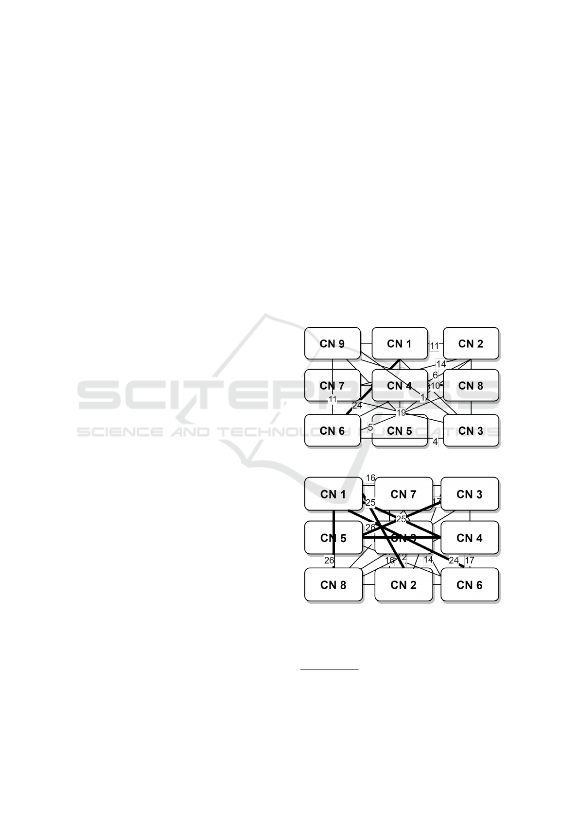
Example 2. We present the weights between the CNs,

of the human cap-dependent 48S pre-initiation com-

plex, in Table 1. To simplify the example the numbers

provided in the table have been scaled down, keeping

the initial ratio. First, we merge the sub-graphs into

one continuous graph, by following the steps of the

proposed algorithm. We present the steps followed as

well as the intermediate results of the cost function in

2. Then, we merge the sub-graphs into one continu-

ous graph in a random way. The results of the two

placements is presented in Figure 1. There is a 40%

decrease to the overall weight cost.

The merged information is stored in a distributed,

scalable Accumulo

key/value datastore where the

GeoMesa

XZ-ordering index is used for the spatial

information of the graph.

(a) Placement based on the proposed algorithm

(b) Random placement

Figure 1: CN Placement in the Two-Dimensional Cartesian

Integer Grid.

https://accumulo.apache.org/

https://www.geomesa.org/documentation/current/

index.html

ICEIS 2020 - 22nd International Conference on Enterprise Information Systems

110

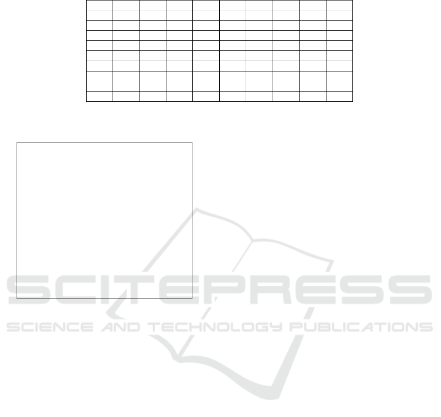
Table 1: Number of External Edges between the Nine CNs.

CN 1 CN 2 CN 3 CN 4 CN 5 CN 6 CN 7 CN 8 CN 9

CN 1 0 25 16 27 3 24 1 26 6

CN 2 25 0 17 24 4 6 14 25 11

CN 3 16 17 0 10 25 17 19 4 1

CN 4 27 24 10 0 26 18 13 12 7

CN 5 3 4 25 26 0 14 27 21 11

CN 6 24 6 17 18 14 0 14 5 11

CN 7 1 14 19 13 27 14 0 10 16

CN 8 26 25 4 12 21 5 10 0 9

CN 9 6 11 1 7 11 11 16 9 0

Table 2: Steps of Executing the Proposed Algorithm for the

Nine CNs.

Step 1 CN 4 is set at the center of the grid

Step 2 CNs are ranked based on the weight [1,5,2,6,7,8,3,9]

Step 3 CN 1 is placed next in the grid

Step 4 CNs are ranked based on the weight [2,6,8,5,3,7,9]

Step 5 CN 2 is placed next in the grid

Step 6 CNs are ranked based on the weight [8,6,3,5,7,9]

Step 7 CN 8 is placed next in the grid

Step 8 CNs are ranked based on the weight [3,6,5,7,9]

Step 9 CN 3 is placed next in the grid

Step 10 CNs are ranked based on the weight [5,6,7,9]

Step 11 CN 5 is placed next in the grid

Step 12 CNs are ranked based on the weight [6,7,9]

Step 13 CN 6 is placed next in the grid

Step 14 CNs are ranked based on the weight [7,9]

Step 15 CN 7 is placed next in the grid

Step 16 CN 9 is placed next in the grid

2.4 Use Cases

In order to provide access to the graph of the input

dataset in an efﬁcient and user-friendly way, we have

implemented a dedicated API that allows the retrieval

of the information in different ways, including spa-

tial and ﬁltering queries and keyword search. We

have implemented a standalone Tomcat application,

written using Java servlets,that receives user requests

along with multiple parameters and returns the result

as an XML ﬁle, that follows the GraphML format and

includes the proper geometry parameters that spec-

ify the position of the nodes in the two-dimensional

space. The API is designed to receive any Common

Query Language function, including all the spatial

functions and geometries. We are going to showcase

the usability of the API through a series of use cases

as identiﬁed in the presented motivating example.

Example 3. Keyword Search. The initial exploration

of the dataset begins when the user wants to locate

information of interest. The intuitive way for this is

to use a keyword and search among the entities of the

dataset. For a protein complex the user may search

the identiﬁer of an atom or a group of atoms. The API

will return a list containing all the entities containing

the given keyword along with their spatial informa-

tion.

Example 4. Spatial Queries. After locating an entity

of interest, the user can use its spatial information and

query the API over the two-dimensional space, using

any Common Query Language spatial function and

geometry. As an example, a user interested in iden-

tifying speciﬁc connections in parts of the biological

structure, responsible for a speciﬁc function, can per-

form spatial queries and retrieve this information.

Example 5. Filtering based on Connection Types.

The API enables the retrieval of the information us-

ing one or multiple ﬁltering criteria at the same time.

The user can easily select to isolate one or more types

of connections between atoms based on their seman-

tic annotations, and can combine this ﬁltering with a

spatial query for a speciﬁc area of the graph.

Example 6. Path Exploration. After locating an en-

tity that is of interest, the user is able to retrieve all the

paths of the graph that include this node, up to a cus-

tomisable length. In contrast to most approaches in

which a path can be traversed only with respect to the

edge direction, in our API when a node is selected, all

neighbors, either incoming or outgoing are retrieved.

3 RELATED WORK

In this section we describe with further details related

work. To begin with, systems that aim to overcome

the restriction of the size limitation based on the ex-

traction of the included information and its represen-

tation through generic visualization options will be

presented.

Facet Graphs (Heim et al., 2010a) allows humans

to access information contained in the Semantic Web

according to its semantics and thus to leverage the

speciﬁc characteristic of this Web. To avoid the am-

biguity of natural language queries, users only select

already deﬁned attributes organized in facets to build

their search queries. The facets are represented as

Efﬁcient Representation of Very Large Linked Datasets as Graphs

111

nodes in a graph visualization and can be interactively

added and removed by the users in order to produce

individual search interfaces. This provides the possi-

bility to generate interfaces in arbitrary complexities

and access arbitrary domains.

SemLens (Heim et al., 2011) is a visual tool that

arranges objects on scatter plots and them using user-

deﬁned semantic lenses, offering visual discovery of

correlations and patterns in data. Haystack (Huynh

et al., 2002) is a platform for creating, organizing and

visualizing information using RDF. It is based on the

idea that aggregating various types of users’ data to-

gether in a homogeneous representation, agents can

make more informed deductions in automating tasks

for users. LODeX (Benedetti et al., 2014) is a tool

that generates a representative summary of a linked

data source. The tool takes as input a SPARQL end-

point and generates a visual summary of the linked

data source, accompanied by statistical and struc-

tural information of the source. Polaris (Stolte and

Hanrahan, 2000) is a visual query language for de-

scribing table-based graphical presentations of data

which compiles into both the queries and the visual-

ization,enabling users to integrate analysis and visu-

alization.

A large number of systems visualize linked

datasets adopting a graph-based approach (Mazumdar

et al., 2015). Most systems, limit the displayed infor-

mation by enforcing a path-based navigation of the

data to the user. Such examples include the RelFinder

(Heim et al., 2010b) which is a web-based tool that

offers interactive discovery and visualization of re-

lationships between selected linked data resources.

Similary, Fenﬁre (Hastrup et al., 2008) and Lodlive

(Camarda et al., 2012) are exploratory tools that allow

users to browse linked data using interactive graph

navigation. Starting from a given URI, the user can

explore linked data by following the links. Zoom-

RDF (Zhang et al., 2010) employs a space-optimized

visualization algorithm in order to display additional

resources with respect to the user navigation choises

while Trisolda (Dokulil and Katreniakov

a, 2009) pro-

poses a clustered RDF graph visualization in which

input information is merged to graph nodes. FlexViz

(Falconer et al., 2010) offers node and edge speciﬁc

ﬁlters that are based on search and navigation crite-

ria aiming to reduce the amount of handled data and

provide to a meaningful subset to the user.

The Tabulator (Berners-Lee et al., 2006) project

is an attempt to demonstrate and utilize the power of

linked RDF data with a user-friendly Semantic Web

browser that is able to recognize and follow RDF links

to other RDF resources based on the user’s explo-

ration and analysis. It is a generic browser for linked

Table 3: Synthetic Datasets.

Dataset #Edges #Nodes Degree

1M D5 5.1M 1M 5.09

10M D5 50.2M 10M 5.02

10M D10 103M 10M 10.3

10M D15 157M 10M 15.7

50M D5 259M 50M 5.18

data on the web without the expectation of provid-

ing as intuitive an interface as a domain-speciﬁc ap-

plication but aiming to provide the sort of common

user interface tools used in such applications, and

to allow domain-speciﬁc functionality to be loaded

transparently from the web and be instantly applica-

ble to any new domain of information. Explorator

(De Araujo and Schwabe, 2009) is an open-source ex-

ploratory search tool for RDF graphs, implemented

in a direct manipulation interface metaphor. It imple-

ments a custom model of operations, and also pro-

vides a Query-by-example interface. Additionally, it

provides faceted navigation over any set obtained dur-

ing the operations in the model that are exposed in the

interface. It can be used to explore both a SPARQL

endpoint as well as an RDF graph in the same way as

“traditional” RDF browsers.

Another approach to the problem of linked data

visualization is the visualization of the information

based on hierarchical models. GrouseFlocks (Ar-

chambault et al., 2007) works only on datasets struc-

tured over well-deﬁned hierarchies. It requires com-

plete data and can handle up to 220K elements when

the hierarchy is predeﬁned. Tulip (Auber, 2004) de-

velops a technique to solve the problem of presenting

to the users the data in only one predetermined way,

regardless of the features of the input dataset. This

tool stores the input data once and extracts the infor-

mation with different techniques providing the user

with multiple views/clusters over the data. GMine (Jr.

et al., 2006) uses the state-of-the-art partitioning algo-

rithm METIS (Karypis and Kumar, 1998) to split the

input dataset in reasonable partitions. Each partition

is visualized as one node, resulting in the loss of the

information included in each partition.

4 EXPERIMENTAL ANALYSIS

In order to evaluate the proposed technique and carry

out an experimental analysis on the efﬁciency of the

information retrieval through the API we developed a

web tool. We used the tool to spatially query the API

and evaluate the response time. The experiments were

conducted using a laptop with an Intel(R) Core(TM)

ICEIS 2020 - 22nd International Conference on Enterprise Information Systems

112

(a) 1M nodes, degree 5 (b) 10M nodes, degree 5

(e) 50M nodes, degree 5

Figure 2: Response Time for Synthetic Datasets.

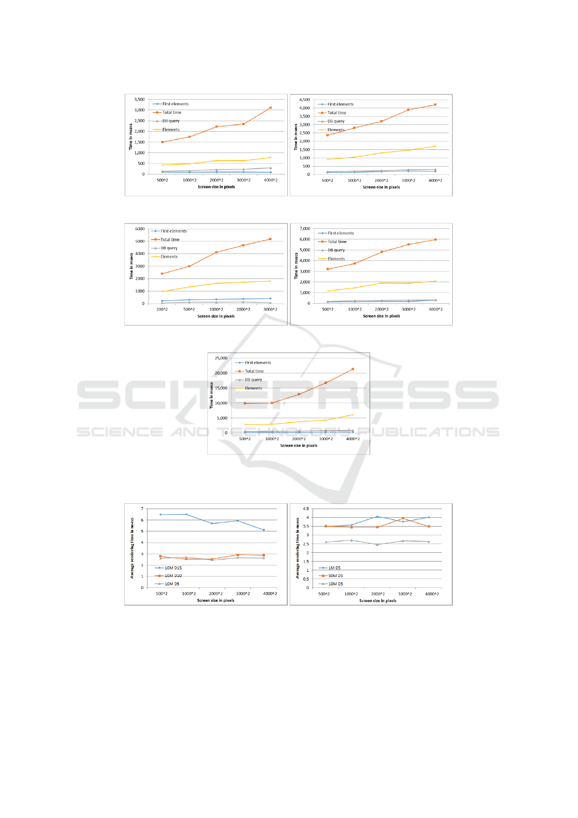
(a) 10M nodes, all degrees (b) degree 5, synthetic datasets

Figure 3: Comparison of Average Response Time per Graph Element.

i7-4500U CPU at 1.80GHz, 4GB RAM memory over

a 12Mbps network connection.

Datasets. In order to test our system with many di-

verse datasets with a wide range of characteristics we

used synthetic datasets. The synthetic datasets, pre-

sented in Table 3, were created to comply with spe-

ciﬁc requirements for number of nodes and node de-

gree to showcase the scalability of the technique to

the size and density as well as the adaptation to any

dataset regardless of its characteristics.

Efﬁcient Representation of Very Large Linked Datasets as Graphs

113

Web Tool Over the Dedicated API. We have imple-

mented a basic web tool for the experimental analysis

of the presented technique. The web tool is based on

the client-server architecture. The server side of the

system is the implementation of the pre-processing

technique as described above, where the input dataset

is transformed into one continuous graph, stored,

indexed and made available through the API. The

client side consists of simple user interface that di-

rectly utilize the API, and depicts the user navigation

actions, such as panning and scrolling, into spatial

queries with respect to the two-dimensional space be-

fore sending the request to the server.

4.1 API Efﬁciency

Metrics. We evaluate the efﬁciency of the technique

based on the time needed to retrieve the nodes from

the API and present them at the web tool after a spatial

query, measured in msecs. The time presented is the

ﬁgures is the time needed for the query execution, the

rendering time for the ﬁrst elements to appear on the

screen and the total response time of the system when

all the elements are rendered.

Methodology. We render randomly selected parts

of the datasets using spatial queries with rectan-

gular bounding boxes ranging from 500x500 px to

4000x4000 px. As the size of the area increases the

spatial queries on the dataset match larger number of

graph elements, allowing us to examine the response

time over a variation of total rendered graph elements.

The experiments present the average results of a series

of one hundred repetitions of the graph rendering for

each rectangle size.

Results. In Figure 2 we present the results for the

synthetic datasets. In all cases the total time is closely

connected to the number of rendered elements. The

system renders more than 500 graph elements in less

than two seconds and up to 5200 graph elements with-

out causing lagging, performance issues or hindering

the user experience, as shown in 2 (e). The fact that

so many graph elements can be rendered smoothly,

is of high importance, as similar systems have lim-

its to the number of presented elements. In Figure 3

we examine the average time needed for the render-

ing of one graph element. In Figure 3 (a) we show

that the average rendering time is not dependent on

the density of the input dataset, while in Figure 3 (b)

we show that it is not dependent on the size of the

input dataset. These experiments prove that our tech-

nique scales efﬁciently for any size or density of the

input dataset and supports the exploration of the in-

formation for datasets with millions of nodes without

any performance issues.

5 CONCLUSIONS

In this paper, we present a novel technique for the pre-

processing very large datasets with hundreds of mil-

lions of elements and their representation as graphs in

the two-dimensional space. Our technique has been

designed in a way to meet all the identiﬁed challenges

regarding exploration needs and user experience. The

presented technique process large real datasets with

millions of elements as well as dense graphs with

high node degree. The technique does not impose

any restrictions on the dataset while the information

is offered through a dedicated API that supports many

functionalities, including keyword search, path explo-

ration and neighbor information.

REFERENCES

Abello, J., van Ham, F., and Krishnan, N. (2006). ASK-

GraphView: A Large Scale Graph Visualization Sys-

tem. TVCG, 12(5).

Archambault, D., Munzner, T., and Auber, D. (2007).

Grouse: Feature-Based, Steerable Graph Hierarchy

Exploration. In EuroVis.

Atemezing, G. A. and Troncy, R. (2014). Towards a linked-

data based visualization wizard. In COLD.

Auber, D. (2004). Tulip - A Huge Graph Visualization

Framework. In Graph Drawing Software.

Benedetti, F., Po, L., and Bergamaschi, S. (2014). A Visual

Summary for Linked Open Data sources. In ISWC.

Berners-Lee, T., Chen, Y., Chilton, L., Connolly, D., Dha-

naraj, R., Hollenbach, J., Lerer, A., and Sheets, D.

(2006). Tabulator: Exploring and analyzing linked

data on the semantic web. In Proceedings of the

3rd international semantic web user interaction work-

shop, volume 2006, page 159. Citeseer.

Brunetti, J. M., Gil, R., and Garc

ıa, R. (2012). Facets and

Pivoting for Flexible and Usable Linked Data Explo-

ration. In Interacting with Linked Data Workshop.

Camarda, D. V., Mazzini, S., and Antonuccio, A.

(2012). LodLive, exploring the web of data. In I-

SEMANTICS.

De Araujo, S. F. and Schwabe, D. (2009). Explorator: a

tool for exploring rdf data through direct manipula-

tion. In Linked data on the web WWW2009 workshop

(LDOW2009).

Dokulil, J. and Katreniakov

a, J. (2009). Using Clusters in

RDF Visualization. In Advances in Semantic Process-

ing.

Falconer, S., Callendar, C., and Storey, M.-A. (2010). A Vi-

sualization Service for the Semantic Web. In Knowl-

edge Engineering and Management by the Masses.

Hastrup, T., Cyganiak, R., and Bojars, U. (2008). Browsing

Linked Data with Fenﬁre. In WWW.

Heim, P., Ertl, T., and Ziegler, J. (2010a). Facet graphs:

Complex semantic querying made easy. In Extended

Semantic Web Conference, pages 288–302. Springer.

ICEIS 2020 - 22nd International Conference on Enterprise Information Systems

114

Heim, P., Lohmann, S., and Stegemann, T. (2010b). Inter-

active Relationship Discovery via the Semantic Web.

In ESWC.

Heim, P., Lohmann, S., Tsendragchaa, D., and Ertl,

T. (2011). SemLens: visual analysis of semantic

data with scatter plots and semantic lenses. In I-

SEMANTICS.

Huynh, D., Karger, D. R., Quan, D., et al. (2002). Haystack:

A platform for creating, organizing and visualizing in-

formation using rdf. In Semantic Web Workshop, vol-

ume 52.

Jr., J. F. R., Tong, H., Traina, A. J. M., Faloutsos, C., and

Leskovec, J. (2006). GMine: A System for Scalable,

Interactive Graph Visualization and Mining. In VLDB.

Kamada, T. and Kawai, S. (1989). An algorithm for draw-

ing general undirected graphs. Information Process-

ing Letters.

Karypis, G. and Kumar, V. (1998). A fast and high qual-

ity multilevel scheme for partitioning irregular graphs.

SIAM J. Sci. Comput., pages 359–392.

ımek, J., Helmich, J., and Necask

y, M. (2013). Payola:

Collaborative Linked Data Analysis and Visualization

Framework. In ESWC.

Mazumdar, S., Petrelli, D., Elbedweihy, K., Lanfranchi, V.,

and Ciravegna, F. (2015). Affective graphs: The visual

appeal of Linked Data. Semantic Web, 6(3).

Oswald, M., Reinelt, G., and Wiesberg, S. (2012). Exact

solution of the 2-dimensional grid arrangement prob-

lem. Discrete Optimization.

Schlegel, K., Weißgerber, T., Stegmaier, F., Seifert, C.,

Granitzer, M., and Kosch, H. (2014). Balloon Syn-

opsis: A Modern Node-Centric RDF Viewer and

Browser for the Web. In ESWC.

Stolte, C. and Hanrahan, P. (2000). Polaris: A Sys-

tem for Query, Analysis and Visualization of Multi-

Dimensional Relational Databases. In InfoVis.

Voigt, M., Pietschmann, S., Grammel, L., and Meißner, K.

(2012). Context-aware Recommendation of Visual-

ization Components. In eKNOW.

Zhang, K., Wang, H., Tran, D. T., and Yu, Y. (2010). Zoom-

RDF: semantic ﬁsheye zooming on RDF data. In

WWW.

Efﬁcient Representation of Very Large Linked Datasets as Graphs

115