Experiments of a New Generation Points Strategy in a Multilocal Method

Amulya Baniya

, Rui Fernandes

2,3

and Florbela P. Fernandes

3 b

Instituto Polit´ecnico de Braganc¸a, Campus de Santa Apol´onia, Braganc¸a, Portugal

Faculdade de Engenharia da Universidade do Porto, Rua Dr. Roberto Frias, Porto, Portugal

Research Centre in Digitalization and Intelligent Robotics (CeDRI), Instituto Polit´ecnico de Braganc¸a,

Campus de Santa Apol´onia, Braganc¸a, Portugal

Keywords:

Points Generation, Derivative-free Method, Multistart, MCSFilter Method, Nonlinear Optimization.

Abstract:

Nonlinear programming problems appear frequently in industrial/real problems. It is important to obtain its

solution in the lowest time possible, since the company could beneﬁt from this. Taking this into account, a

derivative free method (MCSFilter method) is addressed with a different strategy to generate the initial points

to start each local search. The idea is to spread more the points so that the code execution will require a shortest

amount of time when compared with the MCSFilter method execution. Some experiments were performed

with simple bounds problems, equality and inequality constraint problems, chosen from a set of well known

nonlinear problems. The results obtained were encouraging and with the new strategy the method needs less

time to obtain the global solution.

1 INTRODUCTION

Problems coming from different parts in engineering

or economics, among other areas, are very complex

and can be modeled as nonlinear programming prob-

lems (Floudas et al., 1999) or (Hendrix and G.-T´oth,

2010).

Sometimes the derivatives are not known, thus

it is important to use a method that allows us to

solve these problems without this knowledge. The

MCSFilter method is a derivative free method that is

able to treat discontinuous or non-differentiable func-

tions (Fernandes et al., 2013) — a kind of functions

that usually appear in these areas. This method is a

multilocal method meaning that it ﬁnds all the min-

imizers, local and global. The MCSFilter method

was already used to solve small engineering problems

(Amador et al., 2017) or (Amador et al., 2018).

The results obtained with the MCSFilter method

are quite satisfactory, nevertheless, the generation of

initial points is performed randomly. This means that

two or more points can be generated closely to each

other and converge to the same minimizer without

adding new valuable information to the method. The

idea is now to obtain a new strategy, to generate this

points, in such a way that they will be more spread

https://orcid.org/0000-0002-8611-7706

https://orcid.org/0000-0001-9542-4460

around all the search space, leading to a small num-

ber of functions evaluation (or less time) to obtain the

global minimizer. The paper is organized as follows:

in Section 2 a brief description of MCSFilter method

is given; in Section 3 the new strategy to generate the

initial points is presented; in Section 4 the numerical

results are shown and in Section 5 some conclusions

are performed.

2 MCSFilter METHOD

The MCSFilter method is a derivative free method

able to treat nonlinear and constraint problems based

on a multistart strategy coupled with a ﬁlter coordi-

nate search. For more details see (Kolda et al., 2003)

and (Fernandes et al., 2013). The exploration part

of the method is related with the multistart strategy,

meanwhile the exploitation is related with the deriva-

tive free local search procedure CSFilter, in order to

obtain all the solutions (local and global solutions).

The problem can be formulated in the usual way:

min f(x)

subject to g

(x) ≤ 0, j = 1,...,m

≤ x

≤ u

, i = 1,..., n

(1)

where, at least one of the functions f, g

: R

−→ R

is nonlinear and F = {x ∈ R

: g(x) ≤ 0, l ≤ x ≤ u}

Baniya, A., Fernandes, R. and Fernandes, F.

Experiments of a New Generation Points Strategy in a Multilocal Method.

DOI: 10.5220/0009386304030410

In Proceedings of the 9th International Conference on Operations Research and Enterprise Systems (ICORES 2020), pages 403-410

ISBN: 978-989-758-396-4; ISSN: 2184-4372

403

is the feasible region. Problems with general equal-

ity constraints can be reformulated in the above form

by introducing h(x) = 0 as an inequality constraint

|h(x)|−τ ≤ 0, where τ is a small positive relaxation

parameter.

The problem is rewritten as a bi-objective problem

aiming to minimize both, the objective function f(x)

and a nonnegativecontinuous aggregate constraint vi-

olation function θ(x) deﬁned by

θ(x) = kg(x)

+ k(l−x)

+ k(x−u)

(2)

where v

= max{0, v}. Therefore, a minimizer will

be computed by the local search CSFilter to the bi-

objective optimization problem

min

(θ(x), f(x)) . (3)

When a multistart strategy is applied to obtain all

the solutions, some or all of the minimizers may be

found over and over again. To avoid convergence to a

previously computed solution, a clustering technique

based on the regions of attraction computation asso-

ciated with the local search procedure of previously

identiﬁed minimizers, y

, is deﬁned as:

≡ {x ∈[l,u] : CSFilter(x) = y

}, (4)

where CSFilter(x) is the minimizer obtained when

the local search procedure CSFilter starts at point x.

The regions are built and the next local search is

performed, depending (in a probabilistic way) if the

initial point belongs to the region of attraction of some

minimizer found until the moment. The objective of

these regions of attraction is to avoid starting the local

procedure if, for a given point, the local search has a

big probability of converging to some previous deter-

mined minimizers.

Figure 1 illustrates the region of attraction of each

minimizer.

It is possible to see 4 minimizers and the initial

points used for each local search. The red line identi-

ﬁes the ﬁrst local search which converged ﬁrst to each

minimizer; the magenta lines identify all the local

searches that converged to minimizers already found;

the dashed white lines identify all the initial points

that were discarded using the regions of attraction.

To be easier to understand which part is different

from the original version, it is presented the MCSFil-

ter algorithm with the new strategy, related with the

multistart part, Algorithm 1. In this algorithm lines 1,

2 and 5 substitute the random generation of points of

the original MCSFilter algorithm.

As stopping condition, the original MCSFilter al-

gorithm uses the estimate of the fraction of uncovered

space

P(n

min

) =

min

+ 1)

loc

−1)

, (5)

3 4 5 6 7 8 9 10 11 12 13

Figure 1: Regions of attraction of four minimizers.

where n

min

is the number of recovered minimizers

after having performed n

loc

local search procedures.

The multistart algorithm then stops if P(n

min

) ≤ ε, for

a small ε > 0. The CSFilter algorithm is not presented

since it is the same as previously.

All the details about all the parameters inside the

original Algorithm 1 can be seen in (Fernandes et al.,

2013).

3 GENERATION OF INITIAL

POINTS

Taking into account the knowledge about the

MCSFilter algorithm it is possible to state that, with a

big frequency, there are many points generated close

to each other and, on the other side, there are parts

in the search space that do not have any point there.

The idea is to obtain a new way to generate the points

more spread around the search space.

According with (Hedar and Fukushima, 2006) the

interval between the bounds, for each coordinate, is

divided into 4 sub-intervals. In each sub-interval a

value will be generated for each coordinate based on

a probability that depends on which intervals the coor-

dinate has already been generated, and on a dispersion

parameter α ≥ 0, as it can be seen in Algorithm 2.

The number of points to be generated are deﬁned

using 4 different rules. These rules are based in the

search space, given by the bounds and, also, based in

the fact that each interval is dividedinto 4 subintervals

and are deﬁned as follows:

• RGP1: Considering ∆

= u

−l

the number of

points generated (T) is given by:

T =

∏

i=1

⌈∆

⌉, (6)

with ⌈·⌉ being the ceil function.

ND2A 2020 - Special Session on Nonlinear Data Analysis and Applications

404

Algorithm 1: MCSFilter algorithm with a new strategy of

generation of initial points.

Require: Parameter values; set Y

∗

†

, k = 1, t = 1;

1: Generate T points using Algorithm 2;

2: x is the ﬁrst point generated from the T points;

3: Compute y

= CSFilter(x), R

= kx −y

k; set

= 1, Y

∗

= Y

∗

∪y

;

4: repeat

5: x is the next point generated from the T points;

6: Set o = argmin

j=1,...,k

≡ kx−y

7: if d

< R

then

8: if the direction from x to y

is ascent then

9: Set p = 1;

10: else

11: Compute p = ρφ(

);

12: end if

13: else

14: Set p = 1;

15: end if

16: if ζ

‡

< p then

17: Compute y = L(x); set t = t + 1;

18: if ky − y

k > γ

∗

min

, for all j = 1,...,k

then

19: Set k = k+1, y

= y, r

= 1, Y

∗

= Y

∗

∪y

;

compute R

= kx−y

20: else

21: Set R

= max{R

,kx −y

♮

; r

= r

+ 1;

22: end if

23: else

24: Set R

= max{R

,kx −y

k}; r

= r

+ 1;

25: end if

26: until the stopping rule is satisﬁed

—————————————————-

†

- Y

∗

is the set containing the computed minimizers.

‡

- ζ is a uniformly distributed number in (0,1).

- y /∈Y

∗

♮

- ky−y

k ≤ γ

∗

min

• RGP2: Since, for each variable, the interval is

divided into 4 equal parts then:

T = 4

. (7)

• RGP3: In this proposed rule the objective is to

combine both, RGP1 and RGP2:

T = 4(n −1)max(⌈∆⌉). (8)

• RGP4: This rule, the simpler one, is based only

in the number on variables:

T = 10n. (9)

It is also considered that:

• if T ≥ 1500 then T = 1500;

Algorithm 2: Initial Points Generation.

1: Initialization: the number of points T is deﬁned

according with RGP

, j = 1,··· ,4.

2: repeat

3: ∆

= ub

−lb

is divided into 4 equal adjacent

intervals — basic intervals. A counter of num-

ber of occurrences is initialised for these basic

intervals.

4: a starting point is randomly generated within

∆

and its corresponding basic interval number

of occurrences is updated.

5: repeat

6: the current maximum number of points de-

ﬁned in a basic interval, maxOcc, accounted

using all basic intervals is determined.

7: an auxiliar value is computed, by basic in-

terval, according with this rule:

aux(i) = α

maxOcc−Occ(i)

, with i = 1,...,4.

In this equation, Occ(i) represents the num-

ber of points in basic interval i.

8: Exception: if α = 0, for the basic intervals

that have a number of occurrences equal to

the maximum number of occurrences value,

the auxiliar value attributed is 1.

9: a new probability distribution is determined

using the auxiliary values:

prob(i) =

aux(i)

∑

i=1

aux(i)

, with i = 1,...,4.

10: the cumulative probability function of this

probability distribution is determined and is

used as threshold, in conjunction with a new

uniform random number generator that out-

puts values between 0 and 1, to deﬁne the

basic interval of the next point.

11: a random number is generated in the ba-

sic interval identiﬁed in the previous step to

generate the point. Its corresponding num-

ber of occurrences is updated.

12: until all values are deﬁned in a single variable

13: until all values are deﬁned for all the variables

14: assemble ﬁnal points by using the coordinates

previously obtained.

• if T = 1 then T = 10n.

In order to visualize the inﬂuence of the value of

the dispersion parameter α and how it controls the

way the points are generated some remarks about the

algorithm should be made:

• if α = 0, the starting basic interval will always get

a probability of 1 and all others a probability of

0. This implies that the starting basic interval will

have all points — case of greater concentration of

points generation, as depicted in Figure 2.

Experiments of a New Generation Points Strategy in a Multilocal Method

405

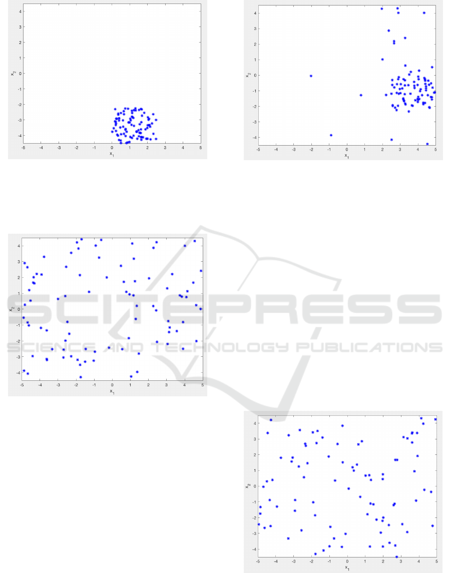
Figure 2: α = 0 and concentration of points.

• if α = 1, all basic intervals will be affected with

the same probability — case of equiprobability

between basic intervals to generate the next point.

One example is presented in Figure 3.

Figure 3: α = 1 and the points spread around the search

space.

• if 0 < α < 1, since aux(i) is a power of α related

to the number of points in the basic interval, inter-

vals with higher number of occurrences will get a

lower power of α, providing them with higher aux

values. A simulation of this scenario can be seen

in Figure 4.

This also means that the probability of achiev-

ing higher concentrated points increases inversely

with the value of α.

• if α > 1, given the relations used, intervals with

lower number of occurrences get higher aux val-

ues. A higher value of α increases more quickly

the value of the exponential distribution used for

the auxiliary values, thus, it implies:

– basic intervals with the maximum number of

occurrences have lower probability of being

Figure 4: α = 0.75 and still a concentration of points.

used in the point generation: higher value of

α ⇒ (more extreme) lower basic interval usage

probability.

– higher value of α, given the higher difference

between different powers of α tends to more

rapidly uniformize the number of occurrences

through all basic intervals. This will render a

situation similar to the case of α = 1 in terms

of points distribution as depicted in Figure 5,

however, there is one important difference be-

tween these two scenario: when α = 1 all inter-

vals are equiprobable, despite the present oc-

currences distribution; when α > 1 intervals

will have different probability values, being

equiprobable, related to the current number of

occurrences. Furthermore, the intervals with

the maximum number of occurrences will have

a much lower probability and this value de-

creases with the increase of the α value.

Figure 5: α = 10 and the points spread around the search

space.

ND2A 2020 - Special Session on Nonlinear Data Analysis and Applications

406

Table 1: Results obtained with the original MCSFilter.

Prob #min

avg

(s)

P1 3 0,1649

P2 5,1 0,1584

P3 3,5 0,3196

P4 2,9 0,2510

P5 2 0,5393

P6 6,7 0,5354

P7 23,5 0,6864

P8 4 0,1434

P9 4 0,1819

P10 8 0,4270

P11 15,6 1,1576

P12 30 3,0336

P13 60,2 7,7436

P14 235 48,5530

P15 1,4 22,9458

P16 3,7 141,1000

4 NUMERICAL RESULTS

To analyze the performance of the MCSFilter algo-

rithm, a set of 16 test problems is used (see Table 6

and the reference therein for more details about each

problem). The set contains bound constrained prob-

lems, inequality and equality constrained problems,

multimodal objective functions, with one global and

some local, more than one global, and a unimodal op-

timization problem.

In order to compare the time needed by the origi-

nal version of the MCSFilter algorithm and the new

one, the original MCSFilter algorithm was run 10

times in a laptop Intel(R) Core i5-7200U CPU and

2.5GHz, using the same values presented in (Fernan-

des et al., 2013). In this version the points are ran-

domly generated and to stop the MCSFilter Algorithm

Equation 5 was used, with ε = 0,1.

These results are listed in Table 1. The ﬁrst col-

umn shows the problems, the second shows the aver-

age number of minimizers found and the last column

shows the average time needed (in seconds).

Tables 2 - 5 list the same results as previously but

now to each new Rule inside Algorithm 2, such that

a comparison can be performed between the original

and the new strategy. Therefore, for each new 4 ways

to limit the generation of the initial points, the average

number of minimizers and the average time needed to

obtain the solutions is presented.

For the proposed MCSFilter algorithm version,

the stop condition is given by Equation 5 or if all T

points are used. All the other parameters remain equal

to the original algorithm. Related with Algorithm 2

Table 2: Results with the RGP1 rule in Algorithm 2.

Prob #min

avg

(s)

P1 3 0,1336

P2 5,7 0,1475

P3 3,9 0,3374

P4 3 0,2445

P5 2 0,4688

P6 7,6 0,6444

P7 21,4 0,6313

P8 4 0,1402

P9 4 0,1549

P10 8 0,3964

P11 15,9 1,0837

P12 31,2 3,0002

P13 61,3 7,7158

P14 235,7 47,8652

P15 1 3,8995

P16 3 15,1904

and the α parameter, after some preliminary experi-

ments it was chosen α = 10.

If a comparison is made between Table 1 and Ta-

ble 2 it is possible to state that using Rule RGP1:

• there are 12 problems out of 16 for which the al-

gorithm takes less time to obtain an equal or larger

number of minimizers;

• there are 2 problems that take more time but the

average numberof minimizers found is larger than

the original;

• for problem P16 it takes less time but the average

number of minimizers (3) is smaller than the av-

erage number (3,7) from the original MCSFilter,

nevertheless the global is always obtained in all

10 runs.

• there is 1 problem in which the results obtained

are worst than the original ones (problem P7).

Considering now Table 3 and Rule RGP2, it is

possible to observe that:

• there are 10 problems out of 16 for which the al-

gorithm takes less time to obtain an equal or larger

number of minimizers;

• there are some problems that take more time but

the average number of minimizers found is larger

than the original.

• for problem P16 the global solution was obtained

only in six runs (out of 10).

To compare the original results with the ones ob-

tained using Rule RGP3, Table 4 lists the average val-

ues to all the problems.

As it is possible to observe:

Experiments of a New Generation Points Strategy in a Multilocal Method

407

Table 3: Results with the RGP2 rule in Algorithm 2.

Prob #min

avg

(s)

P1 3 0,1240

P2 5,7 0,1501

P3 3,7 0,2561

P4 2,9 0,2580

P5 2 0,5681

P6 7,2 0,5330

P7 11,2 0,2198

P8 4 0,1315

P9 4 0,1402

P10 8 0,3907

P11 15,9 1,1509

P12 30,9 2,9382

P13 61,5 7,6835

P14 234,2 50,4519

P15 1 17,5457

P16 2,8 19,4789

Table 4: Results with the RGP3 rule in Algorithm 2.

Prob #min

avg

(s)

P1 3 0,1428

P2 5,4 0,1443

P3 3,9 0,3793

P4 3 0,2013

P5 2 0,4322

P6 6,9 0,4776

P7 21,3 0,6254

P8 4 0,1454

P9 4 0,1531

P10 8 0,4701

P11 15,9 1,1923

P12 30,8 3,0346

P13 60,5 7,7378

P14 167 24,6586

P15 1,3 6,6261

P16 2,8 13,4124

• there are 8 problems out of 16 for which the algo-

rithm takes less time to obtain an equal or larger

number of minimizers;

• there are three problems that take more time but

the average number of minimizers found is larger

than the original.

• for problem P16 the global minimizer was found

only in 5 runs (out of 10).

• for problem P14, the algorithm (with this rule)

found a small number of minimizers, being the

worst result till now, considering all rules.

Finally, Table 5 shows the results obtained with

Rule RGP4.

Comparing these results with Table 1:

Table 5: Results with the RGP4 rule in Algorithm 2.

Prob #min

avg

(s)

P1 3 0,1340

P2 5,5 0,1434

P3 3,7 0,2710

P4 2,8 0,2206

P5 2 0,5082

P6 6,8 0,5034

P7 12,9 0,2428

P8 4 0,1328

P9 4 0,1374

P10 8 0,3804

P11 15,5 0,9803

P12 26,7 1,8912

P13 39,3 3,2597

P14 69,2 7,6520

P15 1,4 15,7886

P16 2,71 14,7141

• there are 10 problems out of 16 for which the al-

gorithm takes less time to obtain an equal or larger

number of minimizers;

• for the remaining problems the results are worst

than the ones obtained with the original algorithm.

• for problem P16 the global minimizer was found

only in 8 runs (out of 10).

Problem P15 has the same behaviour with almost

all rules: ﬁnds a number of minimizers greater than

1. This happen because the local search stops before

reaching the minimizer.

Globally, the MCSFiter algorithm with the mew

points generation strategy needs less time than the

original version to ﬁnd the minimizers, regardless of

the used rule to control the number of points to be

generated, which is promising.

5 CONCLUSIONS

MCSFilter ia a multilocal method able to ﬁnd local

and global solutions of a nonlinear problem. The orig-

inal method is based on a multistart strategy coupled

with a coordinate search ﬁlter methodology. Inside

the multistart part and in the original method, the ini-

tial points were randomly generated. Sometimes, the

points generated were too close of each other leading

to more calls of the local procedure without adding

more information to the solution. The objective of

the new strategy is to spread as much as possible the

points so that it will be possible to avoid some calls

of the local procedure and, hence, taking less time

to obtain the solution. In order to test the efﬁciency

of this approach (Algorithm 2), four different rules

ND2A 2020 - Special Session on Nonlinear Data Analysis and Applications

408

were used to limit the number of points to be gener-

ated. The dispersion or the concentration of the points

around the search space depends on the α parameter.

The new algorithm was tested with all the rules

using, always, a benchmark of test problems — a set

of 16 problems (bound, equality and inequality con-

straint problems).

This preliminary work shows that Algorithm 2

with rules RGP1, RGP2 and RGP4 presents better re-

sults than with RGP3. For bounded problems the re-

sults are better than the original method but the prob-

lems with equality or inequality constraints have a dif-

ferent behaviour.

Currently, the method generates all points ﬁrst and

uses these generated points in MCSFilter algorithm.

That can cause time inefﬁciency for large dimension

problems. Taking this issue into account, individual

point generation, using a similar generation strategy,

should be investigated.

ACKNOWLEDGEMENTS

This work has been supported by FCT — Fundac¸˜ao

para a Ciˆencia e Tecnologia within the Project Scope:

UIDB/5757/2020.

REFERENCES

Amador, A., Fernandes, F. P., Santos, L. O., and Roma-

nenko, A. (2017). Application of mcsﬁlter to esti-

mate stiction control valve parameters. AIP Confer-

ence Proceedings, 1863(1):270005.

Amador, A., Fernandes, F. P., Santos, L. O., Romanenko,

A., and Rocha, A. M. A. C. (2018). Parameter estima-

tion of the kinetic α-pinene isomerization model us-

ing the mcsﬁlter algorithm. In Gervasi, O., Murgante,

B., Misra, S., Stankova, E., Torre, C. M., Rocha, A.

M. A., Taniar, D., Apduhan, B. O., Tarantino, E.,

and Ryu, Y., editors, Computational Science and Its

Applications – ICCSA 2018, pages 624–636, Cham.

Springer International Publishing.

Fernandes, F. P. (2015). Programac¸˜ao n˜ao linear inteira

mista e n˜ao convexa sem derivadas. PhD Thesis, Uni-

versidade do Minho, Braga.

Fernandes, F. P., Costa, M. F. P., and Fernandes, E. M. G. P.

(2013). Multilocal programming: A derivative-free

ﬁlter multistart algorithm. In Murgante, B., Misra,

S., Carlini, M., Torre, C. M., Nguyen, H.-Q., Taniar,

D., Apduhan, B. O., and Gervasi, O., editors, Compu-

tational Science and Its Applications – ICCSA 2013,

pages 333–346, Berlin, Heidelberg. Springer Berlin

Heidelberg.

Floudas, C., Pardalos, P., Adjiman, C., Esposito, W.,

Gumus, Z., Harding, S., Klepeis, J., and Meyer,

C.A.and Schweiger, C. (1999). Handbook of Test

Problems in Local and Global Optimization. Kluwer

Academic Publishers.

Hedar, A.-R. and Fukushima, M. (2006). Derivative-free

ﬁlter simulated annealing method for constrained con-

tinuous global optimization. Journal of Global Opti-

mization, 35(4):521–549.

Hendrix, E. M. T. and G.-T´oth, B. (2010). Introduction to

Nonlinear and Global Optimization. Springer New

York, New York, NY.

Kolda, T. G., Lewis, R. M., and Torczon, V. (2003). Op-

timization by direct search: New perspectives on

some classical and modern methods. SIAM Review,

45(3):385–482.

APPENDIX

The set of problems used to test the new strategy to

generate the initial points were taken from (Fernan-

des, 2015). In Table 6, the ﬁrst column shows the

problem, the second column shows the number of

known minimizers (in the literature), the third column

shows the designation of each problem in (Fernandes,

2015) and the references therein.

Table 6: Information about the problems, number of mini-

mizers and notation.

Prob min known Prob in (Fernandes, 2015)

P1 3 (A.1)

P2 6 (A.2)

P3 4 (A.3)

P4 3 (A.4)

P5 2 (A.5)

P6 10 (A.8)

P7 760 (A.9)

P8 4 (A.11)

P9 4 (A.12)

P10 8 (A.13)

P11 16 (A.14)

P12 32 (A.15)

P13 64 (A.16)

P14 256 (A.17)

P15 1 (A.19)

P16 4 (A.31)

The set of problems used to test the new algorithm

is as follows:

P1:

min f(x) ≡



−

5.1

4π

−6



+10



1−

8π



cos(x

) + 10

s.t −5 ≤x

≤ 10

0 ≤ x

≤ 15

Experiments of a New Generation Points Strategy in a Multilocal Method

409

P2:

min f(x) ≡



4−2.1x



+ x

−4(1−x

s.t −2 ≤x

≤ 2, i = 1,2

P3:

min f(x) ≡ (1+ (x

+ x

+ 1)

(19−14x

+ 3x

−14x

+ 6x

+ 3x

)) ×

×(30+ (2x

−3x

)

×(18−32x

+ 12x

+ 48x

−36x

+ 27x

))

s.t −2 ≤x

≤ 2, i = 1,2

P4:

min f(x) ≡ −

∑

i=1

exp

−

∑

j=1

− p

)

s.t 0 ≤ x

≤ 1,i = 1,2, 3

with

a =







3 10 30

0.1 10 35

3 10 30

0.1 10 35







, c =







1.2

3.2







p =







0.3689 0.117 0.2673

0.4699 0.4387 0.747

0.1091 0.8732 0.5547

0.03815 0.5743 0.8828







P5:

min f(x) ≡ −

∑

i=1

exp

−

∑

j=1

− p

)

s.t 0 ≤ x

≤ 1,i = 1,... ,6

with

a =







10 3 17 3.5 1.7 8

0.05 10 17 0.1 8 14

3 3.5 1.7 10 17 8

17 8 0.05 10 0.1 14







, c =







1.2

3.2







p =







0.1312 0.1696 0.5569 0.0124 0.8283 0.5886

0.2329 0.4135 0.8307 0.3736 0.1004 0.9991

0.2348 0.1451 0.3522 0.2883 0.3047 0.6650

0.4047 0.8828 0.8732 0.5743 0.1091 0.0381







P6:

min f(x) ≡ −−

∑

i=1

(x−a

)(x−a

)

+ c

s.t 0 ≤ x

≤ 10, i = 1,..., 4

with

a =







4 4 4 4

1 1 1 1

8 8 8 8

6 6 6 6

3 7 3 7

2 9 2 9

5 5 3 3

8 1 8 1

6 2 6 2

7 3.6 7 3.6







, c =







0.1

0.2

0.4

0.6

0.3

0.7

0.5







P7:

min f(x) ≡

∑

i=1

icos((i+ 1)x

+ i)

∑

i=1

icos((i+ 1)x

+ i)

s.t −10 ≤ x

≤ 10, i = 1,2

P8:

min f(x) ≡

∑

i=1



sin(x

) + sin





s.t 3 ≤x

≤ 13, 3 ≤ x

≤ 13

P9 (n = 2), P10 (n = 3),

P11 (n = 4), P12 (n = 5),

P13 (n = 6), P14 (n = 8):

min f(x) ≡

∑

i=1

−16x

+ 5x

s.t − 5 ≤x

≤ 5,i = 1,··· ,n

P15:

min f(x) ≡ −(

√

∏

i=1

s.t

∑

i=1

−1 = 0

0 ≤ x

≤ 1,i = 1,··· ,n n = 2

P16:

min f(x) ≡ 4−(x

−1)

−x

s.t (x

+ 5)

+ (x

−5)

−100 ≤ 0

−x

+ 8x

−11 ≤ 0

+ 4x

−7 ≤ 0

+ 4x

−17 ≤ 0

0 ≤ x

≤ 2.5, 0 ≤ x

≤ 2

ND2A 2020 - Special Session on Nonlinear Data Analysis and Applications

410