Evaluating Deep Learning Uncertainty Measures in Cephalometric

Landmark Localization

Dušan Drevický and Old

rich Kodym

Department of Computer Graphics and Multimedia, Brno University of Technology,

Keywords:

Landmark Localization, Cephalometric Landmarks, Deep Learning, Uncertainty Estimation.

Abstract:

Cephalometric analysis is a key step in the process of dental treatment diagnosis, planning and surgery. Local-

ization of a set of landmark points is an important but time-consuming and subjective part of this task. Deep

learning is able to automate this process but the model predictions are usually given without any uncertainty

information which is necessary in medical applications. This work evaluates three uncertainty measures ap-

plicable to deep learning models on the task of cephalometric landmark localization. We compare uncertainty

estimation based on ﬁnal network activation with an ensemble-based and a Bayesian-based approach. We

conduct two experiments with elastically distorted cephalogram images and images containing undesirable

horizontal skull rotation which the models should be able to detect as unfamiliar and unsuitable for automatic

evaluation. We show that all three uncertainty measures have this detection capability and are a viable option

when landmark localization with uncertainty estimation is required.

1 INTRODUCTION

Cephalometric analysis provides clinicians with the

interpretation of the bony, dental and soft tissue struc-

tures in patients’ dental X-ray images. The analysis

results contain relationships between key points in the

radiogram. These landmark positions are then used

for treatment planning, clinical diagnosis, classiﬁca-

tion of anatomical abnormalities and for surgery. This

procedure is time-consuming if performed manually

by experts and high interobserver variability is a sig-

niﬁcant issue as well. Automatic landmark localiza-

tion helps to alleviate both of these problems (Wang

et al., 2016).

The existing solutions for landmark localiza-

tion can be classiﬁed into knowledge-based, pattern

matching-based, statistical learning-based and deep

learning-based. Knowledge-based methods automate

landmark localization by specifying rules based on

expert knowledge (Levy-Mandel et al., 1985). This is

problematic since rule complexity increases propor-

tional with image complexity.

Pattern matching-based methods search for a

speciﬁed pattern within the image. (Cardillo and

Sid-Ahmed, 1994) proposed to use template match-

ing and gray-scale morphological operators. (Grau

et al., 2001) showed that they can improve detection

accuracy by supplementing template matching with

edge detection and contour segmentation operators.

(Davis and Taylor, 1991) used features extracted from

the image to detect a set of candidate positions for

landmarks, and then analyzed the spatial relationships

among landmarks to select the best candidate points.

Statistical learning-based methods take into ac-

count both the local appearance of landmark locations

and global constraints speciﬁed by some model such

as an Active Shape Model (Cootes et al., 1995) or

an Active Appearance Model (Cootes et al., 2006).

Two public challenges for cephalometric landmark

detection were held in 2014 and 2015 at the IEEE

ISBI and the solutions were summarized in (Wang

et al., 2016). Best-performing methods used random

forests for classifying individual landmarks and sta-

tistical shape analysis for capturing the spatial rela-

tionship among landmarks.

Deep learning-based methods have achieved suc-

cess in many application domains and their usage

in medical image analysis has been consistently in-

creasing since 2015 (Litjens et al., 2017). (Payer

et al., 2016) found that convolutional neural networks

(CNNs) can be successful in localizing hand land-

marks. In the context of cephalometric landmark lo-

calization, (Pei et al., 2006) demonstrated the poten-

tial of bimodal deep Boltzmann machines and more

Drevický, D. and Kodym, O.

Evaluating Deep Learning Uncertainty Measures in Cephalometric Landmark Localization.

DOI: 10.5220/0009375302130220

In Proceedings of the 13th International Joint Conference on Biomedical Engineering Systems and Technologies (BIOSTEC 2020) - Volume 2: BIOIMAGING, pages 213-220

ISBN: 978-989-758-398-8; ISSN: 2184-4305

213

recently (Arik et al., 2017) proposed to use deep

CNNs in combination with a shape-based model.

Deep learning-based methods show great poten-

tial but their shortcoming is that they are usually used

as deterministic models providing merely point es-

timates of predictions and model parameters with-

out any associated measure of uncertainty. Since the

models will produce a prediction for any input image,

this may lead to situations in which we cannot tell

whether the prediction is reasonable or just a random

guess (Gal, 2016). That is a problem since informa-

tion about the reliability of model predictions is a key

requirement for their incorporation into the medical

diagnostic systems (Widdowson and Taylor, 2016).

Deep learning models should thus provide each pre-

diction with an estimate of its uncertainty. This would

allow the diagnostic system to distinguish between

easy cases which can be handled automatically and

problematic ones which may instead be referred to a

supervising physician for review.

Models based on probability and uncertainty have

been extensively studied in the Bayesian machine

learning community. They provide a probabilistic

view that offers conﬁdence bounds when performing

decision making (Gal, 2016) but usually come with

a prohibitive computational cost. To take advantage

of the qualities of deep learning models and still have

the option of assessing the uncertainty of their pre-

dictions, it has been suggested (Gal and Ghahramani,

2016) to recast them as Bayesian models using the

popular dropout (Hinton et al., 2012) technique often

used for regularization in neural networks. The poste-

rior distribution used by Bayesian models is approx-

imated in deep learning models using Monte Carlo

(MC) sampling and model uncertainty is given by the

prediction variance of the samples. The MC Dropout

method has already been applied in medical imag-

ing applications. (Leibig et al., 2017) used dropout-

based uncertainty when diagnosing diabetic retinopa-

thy from fundus images. (Eaton-Rosen et al., 2018)

and (Guha Roy et al., 2018) both applied it to seman-

tic segmentation of brain scan images.

Another option for estimating the uncertainty of

deep learning models comes from a recent non-

Bayesian line of research by (Lakshminarayanan

et al., 2017). While ensembles of machine learn-

ing models have long been known to increase per-

formance in terms of predictive accuracy, the authors

also suggest using the prediction variance of the en-

semble members as measure of the ensemble’s uncer-

tainty.

While (Gal, 2016) criticized the use of raw model

outputs as a measure of uncertainty estimation, that

conclusion was not based on experiments conducted

on a heatmap regression task (Payer et al., 2016).

Since we use that method to localize cephalometric

landmarks in this work, we also determine whether a

useful uncertainty measure can be derived from the

predictions of a CNN trained for the task of heatmap

regression.

The contribution of our work is in evaluating the

MC Dropout and ensemble methods of estimating

deep learning model uncertainty on the cephalometric

landmark localization task. To the best of our knowl-

edge, deep learning model uncertainty estimation has

not been studied on this task before. We further eval-

uate whether CNN activations can be used for esti-

mation of landmark uncertainty without multiple for-

ward passes required by other methods. We show that

all three uncertainty measures are able to detect out-

of-distribution data unsuitable for automatic evalua-

tion. Our experiments also hint at the possibility of

applying models trained on X-ray images to 2D CT

projections.

2 MATERIALS AND METHODS

2.1 Dataset

The dataset used for the landmark localization exper-

iments was released as a part of the 2014 and 2015

IEEE ISBI challenges (Wang et al., 2016). It consists

of 400 cephalograms from 400 subjects. All cephalo-

grams were acquired in the same format and from an

identical scanning machine. The resolution of the im-

ages is 1935 x 2400 pixels with a pixel spacing of 0.1

mm. Two orthodontists provided ground truth manual

annotations of 19 cephalometric landmark positions

and we used only the one from the senior physician

accuracy evaluation. For consistency with the proto-

col designed for the competition, we used only 150

images for training and the rest (which is split by the

competition authors into split test1 and test2) for eval-

uation.

2.2 Landmark Localization

We implemented landmark localization using

heatmap regression (Payer et al., 2016). In this

approach, the landmark positions are not regressed

directly as a pair of real coordinates but the model

learns to regress a separate heatmap for each land-

mark instead. For each training example, the CNN

receives a single-channel gray-scale image rescaled

to d × d dimensions. The corresponding ground truth

is a 19 × d × d volume of heatmaps. Each heatmap

corresponds to a single landmark and contains a

BIOIMAGING 2020 - 7th International Conference on Bioimaging

214

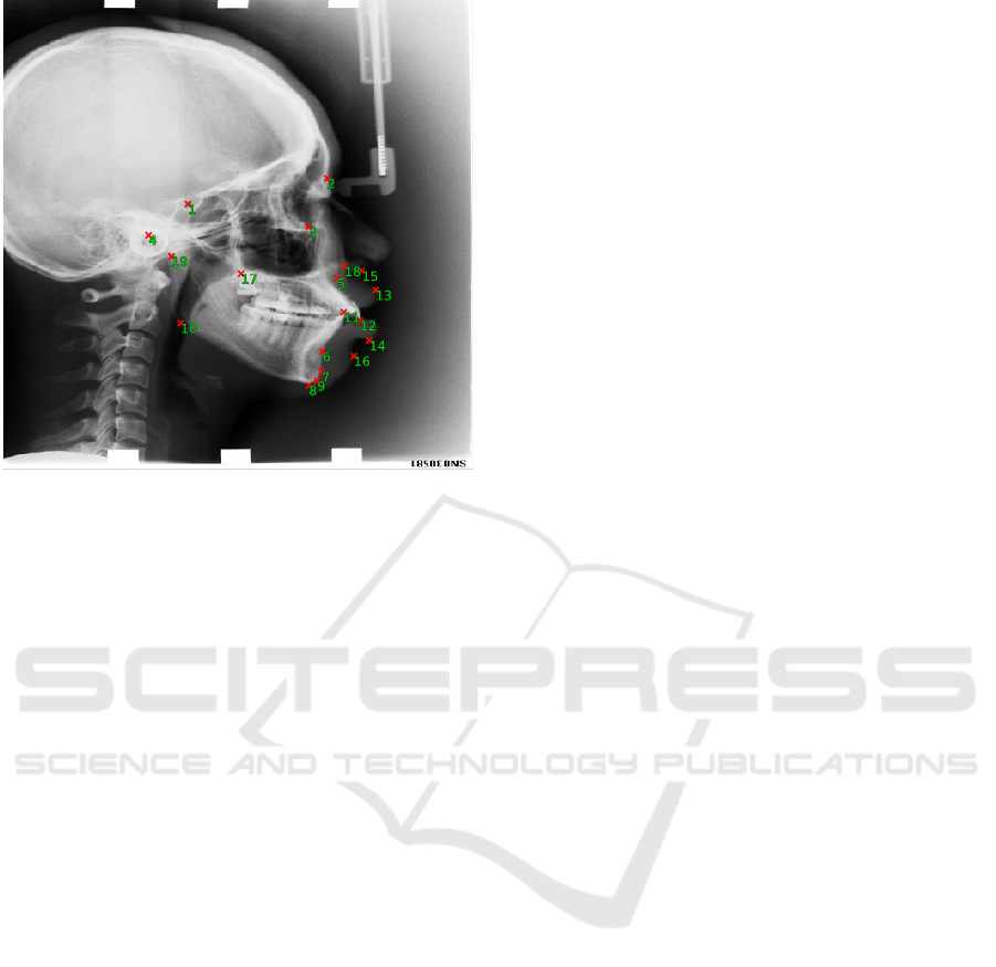
Figure 1: A rescaled image from the 2015 IEEE ISBI chal-

lenge dataset with 19 ground truth landmarks visualized.

Gaussian with a ﬁxed variance and amplitude cen-

tered on the landmark position as annotated by the

physician. The output of the CNN is a 19 × d × d

volume of predicted heatmaps minimizing the mean

squared error loss. As a post-processing step, each

heatmap is convolved with a Gaussian ﬁlter of the

same variance as was used when creating the ground

truth heatmap. The position of the maximum value

in this activation map is chosen as the ﬁnal predicted

landmark position.

2.3 CNN Architecture

The CNN architecture we used closely follows the

U-Net (Ronneberger et al., 2015) with some minor

modiﬁcations. U-Net contains a down-sampling path

followed by a symmetric up-sampling path and is de-

signed to be able to learn both global context (relative

landmark positions) and local characteristics of each

landmark.

The down-sampling path contains 3 × 3 double

convolutions with ﬁlter sizes of 64, 128, 256, 512 and

1024, each followed by a 2 × 2 max pooling layer.

Width and height of the feature map are then progres-

sively increased back to the original 128 ×128 size in

the up-sampling path via transpose convolution which

halves the ﬁlter dimension. Feature map from the cor-

responding down-sampling level is concatenated to

the result and this is followed by a double convolu-

tion whose ﬁlter size decreases from the bottom level

towards the top (1024, 512, 256, 128 and 64). The

ﬁnal double convolution uses 19 ﬁlters to produce the

prediction heatmaps.

For the model based on Monte Carlo dropout (see

Section 2.4.3), dropout layers are added just before

each max pooling layer and right after the transposed

convolution in the up-sampling path.

2.4 Uncertainty Measures

We train three models, all based on the same CNN

architecture. Baseline model uses the activation

heatmap produced by the CNN when estimating un-

certainty while the Ensemble and MC-Dropout mod-

els both use prediction variance of the ensemble mem-

bers and MC samples respectively.

2.4.1 Maximum Heatmap Activation (MHA)

Baseline is a single CNN without dropout layers. Re-

call from Section 2.2 that the heatmap predicted by

the CNN is convolved with a Gaussian ﬁlter as a post-

processing step. The position of the maximum value

in the activation map produced this way is chosen as

the predicted landmark position. The Baseline model

additionally uses the maximum activation value (not

just the position) as a measure of uncertainty associ-

ated with the prediction. We hypothesized that there

is an inverse correlation between the maximum acti-

vation and the uncertainty of the model. The CNN is

trained to output a heatmap which has a strong maxi-

mum at the correct position. Consequently, when the

predicted maximum is low, it might be a good indi-

cator that the network is not sure about the predic-

tion. Note that maximum heatmap activation (MHA)

is technically a measure of model certainty since it

should increase proportional to model’s conﬁdence in

its predictions.

For the purpose of experiment analysis in Sec-

tion 3, this quantity was normalized to a unit range.

The upper bound of one for normalization was cho-

sen based on the maximum value of this uncertainty

measure observed for all of the landmarks in the test

set. Note that the other two models described in this

section ignore the value of the MHA (and only use its

position) and do not use it for uncertainty estimation.

2.4.2 Ensemble Prediction Variance

Ensemble is an ensemble model consisting of 15

CNNs trained independently using the same CNN ar-

chitecture as the Baseline model. To predict landmark

positions for an input image, each CNN in the ensem-

ble is ﬁrst evaluated as described in Section 2.2 and

produces its individual predictions of the landmark

positions. Predictions of all networks are then aver-

aged to produce the ﬁnal position (see Equation 1).

While it is well-known that forming an ensemble of

Evaluating Deep Learning Uncertainty Measures in Cephalometric Landmark Localization

215

machine learning models improves prediction accu-

racy, (Lakshminarayanan et al., 2017) suggested treat-

ing the variance of the ensemble members’ predic-

tions (see Equation 2) as a measure of uncertainty.

Greater variance indicates discord in the ensemble

predictions. The member models were trained using

random initialization so they all ended up with dif-

ferent parameter values at the end of training. Since

they were trained using the same data, it is reasonable

to assume that there will not be a large difference be-

tween their predictions on data coming from a similar

distribution like the one they observed during train-

ing. On the other hand, when being evaluated on out-

of-distribution data (such as a misaligned X-ray, or

an X-ray from a different scanner) the difference be-

tween predictions will be larger since each model will

take a different guess on the unfamiliar data based on

its ﬁnal parameters.

2.4.3 Monte Carlo Dropout Prediction Variance

The Monte Carlo (MC) Dropout technique is based

on the Bayesian assumption that neural network

weights W have probability distributions instead of

being point estimates as is common in deep learn-

ing. The goal of Bayesian modelling is to approxi-

mate the posterior distribution p(W|X, Y) given the

training data {X,Y}. While true Bayesian neural

networks are computationally expensive, (Gal and

Ghahramani, 2016) suggested approximating them

with dropout (Hinton et al., 2012). When applying a

dropout layer in a CNN, a randomly selected subset of

neurons in the previous layer is dropped at each itera-

tion. Since the number of CNN parameters is usually

in the millions, this essentially leads to a different net-

work being sampled at each iteration. The resulting

stochasticity of the network can be used to approxi-

mate a Bayesian neural network. In practice, evalu-

ating the prediction of a an MC Dropout based net-

work amounts to computing the mean of T stochas-

tic forward passes through the network, which sam-

ple from T network architectures (different neurons

are dropped for each one). The predictive uncertainty

over a prediction is obtained by computing the sample

variance of the T forward passes.

2.4.4 Prediction Mean and Prediction Variance

The Ensemble and MC-Dropout models both use pre-

diction variance as a measure of their uncertainty. For

the task of landmark localization, we compute the pre-

diction variance of a vector~y containing T prediction

samples as the mean Euclidean distance between the

prediction samples y

and the prediction mean ˆy:

ˆy =

∑

i=1

(1)

Var(~y) =

∑

i=1

− ˆyk (2)

Note that the prediction mean ˆy is also used as

the landmark location predicted by the Ensemble and

MC-Dropout models.

2.5 Implementation Details

All training images were resized to 128 × 128 size to

speed up training and allow for faster experimenta-

tion. The predictions and prediction variance of the

Ensemble and MC-Dropout models was computed

using 15 ensemble CNNs and MC samples respec-

tively. The probability of a unit being dropped in the

MC-Dropout model was set uniformly to p = 0.4. All

models along with the training process were imple-

mented using the PyTorch (Paszke et al., 2017) li-

brary.

3 EXPERIMENTS AND RESULTS

We ﬁrst shortly evaluate the landmark localization ac-

curacy of the trained models. We then describe two

experiments which aimed to assess whether the eval-

uated uncertainty measures are able to reliably detect

out-of-distribution data on the cephalometric land-

mark localization task.

3.1 Landmark Localization Accuracy

We ﬁrst veriﬁed that the performance of our models

was comparable to that of the best previous solutions

on the dataset we used (see Table 1). Due to compu-

tational reasons, we trained on images resized to the

128 × 128 size from the original 1935 × 2400. While

it was sufﬁcient for the purpose of our study, image

sub-sampling reduced the accuracy of the models and

direct clinical application would require it to be less

aggressive.

3.2 Elastically Distorted

Out-of-Distribution Data Detection

Elastic distortion was applied to the entire test set to

evaluate the ability of the uncertainty measures to de-

tect out-of-distribution data examples. Forty versions

of the test set were created in total, and each copy had

an elastic distortion of progressively stronger mag-

nitude applied to it. First row in Figure 2 shows a

BIOIMAGING 2020 - 7th International Conference on Bioimaging

216

λ=0

λ=70

λ=140

λ=200

θ=0°

θ=15°

θ=30°

θ=45°

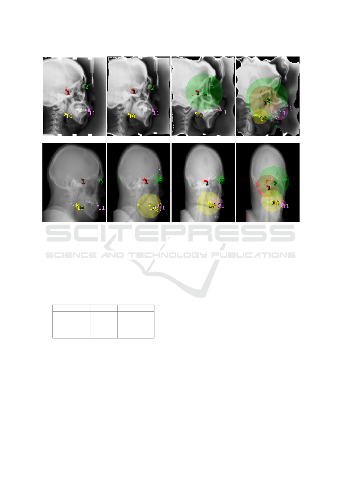
Figure 2: Visualization of the Ensemble model’s predictions and uncertainty values. Top row shows an image from the test

set transformed with elastic distortion of increasing magnitude λ. Bottom row shows a skull CT scan rotated in the horizontal

plane by angle θ and projected onto the sagittal plane. The individual ensemble members’ predictions (dots) are combined

into a ﬁnal position prediction (star), and the ground truth is marked by a cross (only applicable to the top left undistorted

image with known ground truth). Only four landmarks are shown for clarity. As the magnitude of elastic distortion and

rotation increases, so does the model uncertainty (prediction variance).

Table 1: Accuracy of the proposed models on the test1 split

compared with the best solution from the 2015 IEEE ISBI

challenge (Wang et al., 2016). Mean Radial Error gives the

mean error in landmark detection. Success Detection Rate

gives the percentage of predictions within that radius of the

ground truth.

MRE SDR 2.5 mm

Lindner et al. 1.67 mm 80.2 %

Baseline 2.05 mm 74.4 %

Ensemble 1.79 mm 78.5 %

MC-Dropout 1.92 mm 74.7 %

test image transformed with an elastic distortion of

varying strength, along with the landmark predictions

of the Ensemble model for that image. Uncertainty

for each predicted landmark position (variance of the

prediction samples) is visualized by a circle superim-

posed upon the predicted location.

Each model’s predictions and uncertainty esti-

mates for every version of the distorted test set was

then computed. Left column in Figure 3 shows the

correlation between the mean uncertainty measure

value for all landmark position predictions for a given

version of the test set, and the elastic distortion mag-

nitude applied to that version of the test set. The anal-

ysis shows that a strong correlation exists between

the mean value of each uncertainty measure and the

strength of the elastic distortion being applied on the

data.

3.3 Rotated Out-of-Distribution Data

Detection

During the process of X-ray scanning for the purpose

of cephalometric analysis, patient’s head in the scan-

ner should be perfectly aligned with the sagittal plane.

However, patients sometimes rotate their head in the

horizontal plane which distorts the resulting image

and may even lead to some of the landmarks over-

lapping. A model should detect such data by being

uncertain about its predictions.

Since a dataset of cephalograms containing hori-

zontal head rotation is not publicly available, we used

a volumetric CT scan of a single skull to create one.

Evaluating Deep Learning Uncertainty Measures in Cephalometric Landmark Localization

217

0 25 50 75 100 125 150 175 200

Elastic Distortion Magnitude

0.3

0.4

0.5

0.6

0.7

Mean Heatmap Activation

= -0.95

Baseline

0 10 20 30 40

Skull Rotation (°)

0.1

0.2

0.3

0.4

0.5

0.6

0.7

Mean Heatmap Activation

= -0.91

Baseline

0 25 50 75 100 125 150 175 200

Elastic Distortion Magnitude

0.0

2.5

5.0

7.5

10.0

12.5

15.0

17.5

Mean Prediction Variance (mm)

= 0.81

Ensemble

0 10 20 30 40

Skull Rotation (°)

Mean Prediction Variance (mm)

= 0.95

Ensemble

0 25 50 75 100 125 150 175 200

Elastic Distortion Magnitude

Mean Prediction Variance (mm)

= 0.85

MC-Dropout

0 10 20 30 40

Skull Rotation (°)

Mean Prediction Variance (mm)

= 0.88

MC-Dropout

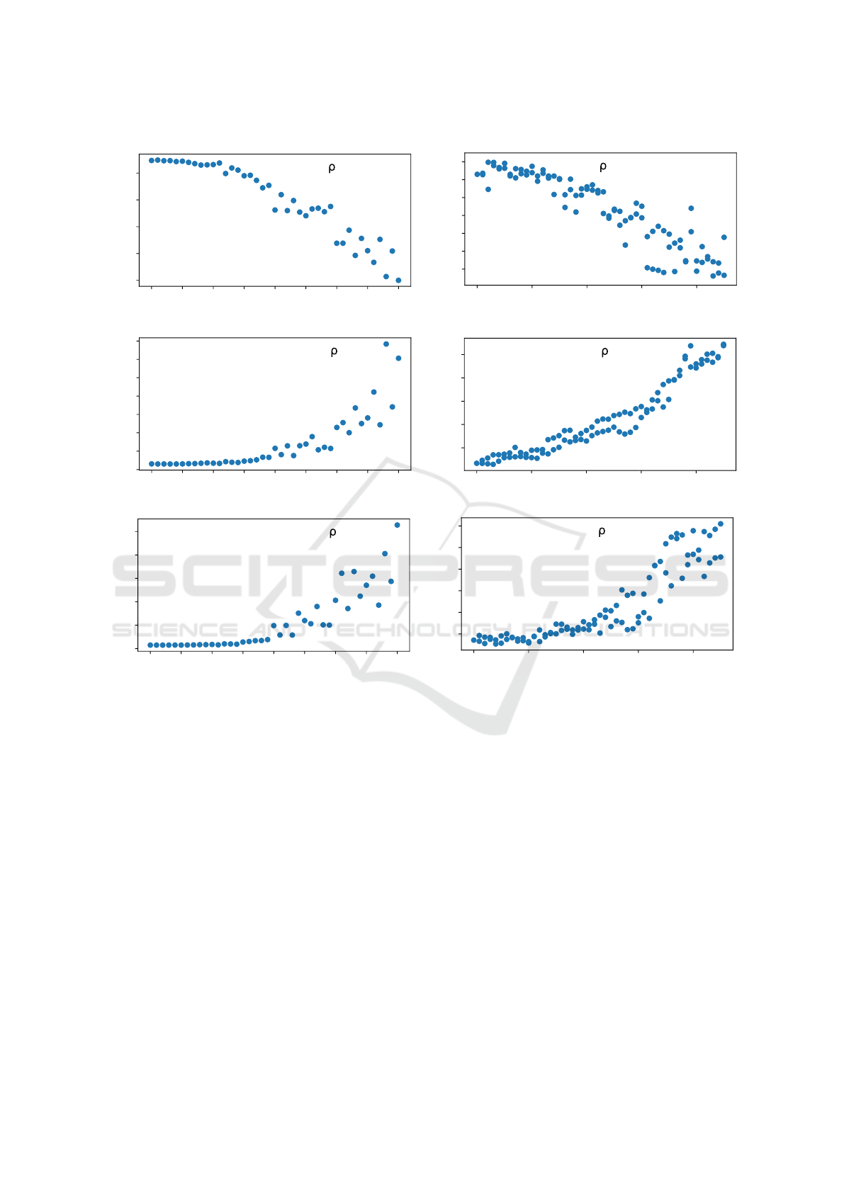
Figure 3: Correlation of the three uncertainty measure values with elastic distortion magnitude (left) and skull rotation mag-

nitude (right). In the ﬁrst experiment, each of the models along with its uncertainty measure was evaluated on forty versions

of the test set modiﬁed by elastic distortion of varying magnitude. In the second experiment, the models were evaluated on

91 images of a skull CT scan projected onto the sagittal plane. The skull was transformed before projection with different

magnitudes of rotation. As distortion and rotation magnitude increase, so does model uncertainty for all three measures. Note

that maximum heatmap activation (top row) is actually a measure of model certainty so the correlation is negative as expected.

The skull volume (originally aligned with the sagit-

tal plane) was ﬁrst rotated by θ degrees in the hori-

zontal plane to simulate a patient’s undesirable move-

ment in the scanner. To simulate X-ray acquisition

process, the resulting volume was then projected onto

the sagittal plane by summing the intensity values of

overlapping voxels. Pixel values in the resulting 2D

image were then normalized by dividing them with

the maximum pixel intensity present in the image.

The resulting dataset contains 91 images with θ rang-

ing from −45° to 45° including a rotation of 0°.

We ﬁrst veriﬁed that the model predictions for the

CT volume projection without any rotation were rea-

sonably accurate. The models provided acceptable

predictions but their mean uncertainty increased com-

pared with the predictions from the X-ray images in

the test set (compare the model uncertainty in the ﬁrst

image in the top row with the ﬁrst image in the bottom

row of Figure 2). This is not unexpected since even

a CT projection created from an unrotated skull vol-

ume is an out-of-distribution data point for a network

trained on X-ray images. However, the sensible pre-

dictions of the models indicate that it is plausible to

apply X-ray trained models on CT projections with-

out a substantial loss of performance. A more con-

ﬁdent conclusion would require further research us-

ing more CT scans. Also note that the viability of

an inverse knowledge transfer (i.e., applying models

BIOIMAGING 2020 - 7th International Conference on Bioimaging

218

trained on CT projections to X-ray data) was previ-

ously observed by (Bier et al., 2018).

The models’ prediction and uncertainty measure

values were then evaluated for each image in the cre-

ated dataset. Right column in Figure 3 shows the

correlation between the mean uncertainty value for

a given image (computed as the mean of uncertainty

estimates for all of the landmarks predicted for the

image) and the magnitude of rotation corresponding

to that image. For each evaluated uncertainty mea-

sure, there is a very strong correlation with the rota-

tion magnitude.

It is noteworthy that the ensemble uncertainty in-

creases more stably than MHA uncertainty as the ro-

tation applied to the image intensiﬁes. For most steps

in rotation increase (an increase of 1°, e.g., from

10° to 11°), there is a corresponding increase in un-

certainty. Additionally, this increase has a consistent

magnitude between all rotation steps. On the other

hand, the MHA uncertainty values increase on the

whole, but the difference in the uncertainty values be-

tween successive rotation steps oscillates. Moreover,

for some consecutive rotation steps, the MHA uncer-

tainty actually decreases signiﬁcantly for such a small

change in the input image. The MC Dropout method

suffers from a similar instability.

We hypothesize that the superior stability of the

ensemble prediction variance is due to the fact that the

Ensemble model consists of 15 unique CNNs while

the other two measures only have a single CNN avail-

able. A single network might have a weak spot in

its parameters for some inputs, which then also af-

fects the associated uncertainty estimate. Multiple

networks will possibly different weak spots and the

average of their predictions will be more reasonable

which will positively affect uncertainty estimate as

well.

A visualization of the Ensemble model’s predic-

tions and corresponding uncertainty values for a skull

projection rotated by different angle θ are in the bot-

tom row of Figure 2.

4 CONCLUSION

In this paper, we evaluated three measures for estimat-

ing deep learning model uncertainty on the cephalo-

metric landmark localization task. We compared un-

certainty estimation based on the maximum heatmap

activation (MHA) of a heatmap regression CNN with

an ensemble-based and a Bayesian-based approach.

Our experiments with out-of-distribution data

showed a strong correlation between the uncertainty

estimates accompanying model predictions and the

distance of the data from the training distribution for

all measures. This suggests their usability in detect-

ing images unsuitable for automatic evaluation. When

individually comparing the measures’ performance,

MHA showed the strongest correlation with image

distance from training distribution when both exper-

iments are taken into account. On the other hand,

both MHA and the MC Dropout uncertainty values

increased inconsistently in the rotation experiment

while the ensemble uncertainty was very stable in this

regard.

The usability of MHA is an interesting ﬁnding be-

cause this uncertainty measure is directly available

when using a CNN trained for heatmap regression.

Conversely, the other two measures require the model

to contain dropout layers or necessitate the training

of multiple networks. Additionally, while MHA re-

quires a single forward pass of the image, the other

examined methods both need multiple passes and are

more computationally expensive.

Although MHA could be used as a strong baseline

uncertainty estimation method on its own, due to its

observed instability it might be useful to combine it

(e.g., by a weighted average) with one of the ensem-

ble (preferrably) or MC Dropout methods when their

requirements and the increase in computation time are

not a problem.

To further verify that the uncertainty measures we

explored in this work are able to detect the failure

cases when a model is being applied on data distant

from its training distribution, it would be desirable

to train the CNN on cephalograms from one set of

scanners and then evaluate it on images from a dif-

ferent set of scanners. Another experiment could tar-

get a more conﬁdent result regarding the potential of

applying X-ray trained deep learning models on CT

projection images by using a larger dataset of CT vol-

umes. Since this issue is not necessarily restricted to

cephalometry or landmark localization, it would also

be preferable to expand the experiments to include

other machine learning tasks and other type of struc-

tures beside skulls.

ACKNOWLEDGEMENTS

This work was supported by the company

TESCAN 3DIM. We would also like to thank

the same company for providing us with the CT data

used in the experiments.

Evaluating Deep Learning Uncertainty Measures in Cephalometric Landmark Localization

219

REFERENCES

Arik, S., Ibragimov, B., and Xing, L. (2017). Fully

automated quantitative cephalometry using convolu-

tional neural networks. Journal of Medical Imaging,

4:014501.

Bier, B., Unberath, M., Zaech, J.-N., Fotouhi, J., Armand,

M., Osgood, G., Navab, N., and Maier, A. (2018).

X-ray-transform invariant anatomical landmark de-

tection for pelvic trauma surgery. In Frangi, A. F.,

Schnabel, J. A., Davatzikos, C., Alberola-López, C.,

and Fichtinger, G., editors, Medical Image Computing

and Computer Assisted Intervention – MICCAI 2018,

pages 55–63, Cham. Springer International Publish-

ing.

Cardillo, J. and Sid-Ahmed, M. A. (1994). An image pro-

cessing system for locating craniofacial landmarks.

IEEE Transactions on Medical Imaging, 13(2):275–

289.

Cootes, T., Edwards, G., and Taylor, C. (2006). Active ap-

pearance models, volume 23, pages 484–498.

Cootes, T., Taylor, C., Cooper, D., and Graham, J.

(1995). Active shape models-their training and appli-

cation. Computer Vision and Image Understanding,

61:38–59.

Davis, D. N. and Taylor, C. (1991). A blackboard architec-

ture for automating cephalometric analysis. Medical

informatics = Médecine et informatique, 16:137–49.

Eaton-Rosen, Z., Bragman, F., Bisdas, S., Ourselin, S., and

Cardoso, M. J. (2018). Towards Safe Deep Learn-

ing: Accurately Quantifying Biomarker Uncertainty

in Neural Network Predictions: 21st International

Conference, Granada, Spain, September 16–20, 2018,

Proceedings, Part I, pages 691–699.

Gal, Y. (2016). Uncertainty in Deep Learning. PhD thesis,

University of Cambridge.

Gal, Y. and Ghahramani, Z. (2016). Dropout as a bayesian

approximation: Representing model uncertainty in

deep learning. In Proceedings of the 33rd Inter-

national Conference on International Conference on

Machine Learning - Volume 48, ICML’16, pages

1050–1059. JMLR.org.

Grau, V., Alcañiz Raya, M., Juan, M.-C., Monserrat, C., and

Knoll, C. (2001). Automatic localization of cephalo-

metric landmarks. Journal of biomedical informatics,

34:146–56.

Guha Roy, A., Conjeti, S., Navab, N., and Wachinger, C.

(2018). Inherent Brain Segmentation Quality Con-

trol from Fully ConvNet Monte Carlo Sampling, pages

664–672.

Hinton, G. E., Srivastava, N., Krizhevsky, A., Sutskever,

I., and Salakhutdinov, R. (2012). Improving neural

networks by preventing co-adaptation of feature de-

tectors. CoRR, abs/1207.0580.

Lakshminarayanan, B., Pritzel, A., and Blundell, C. (2017).

Simple and scalable predictive uncertainty estimation

using deep ensembles. In Guyon, I., Luxburg, U. V.,

Bengio, S., Wallach, H., Fergus, R., Vishwanathan, S.,

and Garnett, R., editors, Advances in Neural Informa-

tion Processing Systems 30, pages 6402–6413. Curran

Associates, Inc.

Leibig, C., Allken, V., Ayhan, M. S., Berens, P., and Wahl,

S. (2017). Leveraging uncertainty information from

deep neural networks for disease detection. Scientiﬁc

Reports, 7.

Levy-Mandel, A. D., Tsotsos, J. K., and Venetsanopou-

los, A. N. (1985). Knowledge-based landmarking of

cephalograms. In Lemke, H., Rhodes, M. L., Jaffee,

C. C., and Felix, R., editors, Computer Assisted Ra-

diology / Computergestützte Radiologie, pages 473–

478, Berlin, Heidelberg. Springer Berlin Heidelberg.

Litjens, G. J. S., Kooi, T., Bejnordi, B. E., Setio, A. A. A.,

Ciompi, F., Ghafoorian, M., van der Laak, J., van Gin-

neken, B., and Sánchez, C. I. (2017). A survey on

deep learning in medical image analysis. Medical im-

age analysis, 42:60–88.

Paszke, A., Gross, S., Chintala, S., Chanan, G., Yang, E.,

DeVito, Z., Lin, Z., Desmaison, A., Antiga, L., and

Lerer, A. (2017). Automatic differentiation in pytorch.

In NIPS-W.

Payer, C., Stern, D., Bischof, H., and Urschler, M. (2016).

Regressing Heatmaps for Multiple Landmark Local-

ization Using CNNs, volume 9901 of Lecture Notes in

Computer Science, pages 230–238. Springer Interna-

tional Publishing AG, Switzerland.

Pei, Y., Liu, B., Zha, H., Han, B., and Xu, T. (2006).

Anatomical structure sketcher for cephalograms by bi-

modal deep learning. Trans. Biomed. Eng., 53:1615–

1623.

Ronneberger, O., Fischer, P., and Brox, T. (2015). U-

net: Convolutional networks for biomedical image

segmentation. In Navab, N., Hornegger, J., Wells,

W. M., and Frangi, A. F., editors, Medical Image Com-

puting and Computer-Assisted Intervention – MICCAI

2015, pages 234–241, Cham. Springer International

Publishing.

Wang, C.-W., Huang, C.-T., Lee, J.-H., Li, C.-H., Chang,

S.-W., Siao, M.-J., Lai, T.-M., Ibragimov, B., Vrtovec,

T., Ronneberger, O., Fischer, P., Cootes, T. F., and

Lindner, C. (2016). A benchmark for comparison of

dental radiography analysis algorithms. Medical Im-

age Analysis, 31:63 – 76.

Widdowson, S. and Taylor, D. (2016). The management of

grading quality: good practice in the quality assurance

of grading. Tech Report.

BIOIMAGING 2020 - 7th International Conference on Bioimaging

220