Comparing Machine Learning Techniques for Malware Detection

Joanna Moubarak and Tony Feghali

Potech Labs, Beirut, Lebanon

Keywords:

Malware Analysis, Data Science, Machine Learning, Detection, Malicious Behavior.

Abstract:

Cyberattacks and the use of malware are more and more omnipresent nowadays. Targets are as varied as states

or publicly traded companies. Malware analysis has become a very important activity in the management

of computer security incidents. Organizations are often faced with suspicious ﬁles captured through their

antiviral and security monitoring systems, or during forensics analysis. Most solutions funnel out suspicious

ﬁles through multiple tactics correlating static and dynamic techniques in order to detect malware. However,

these mechanisms have many practical limitations giving rise to a new research track. The aim of this paper

is to tackle the use of machine learning algorithms to analyze malware and expose how data science is used to

detect malware. Training systems to ﬁnd attacks allows to develop better protection tools, capable of detecting

unprecedented campaigns. This study reveals that many models can be employed to evaluate their detectability.

Our demonstration results illustrates the possibility to analyze malware leveraging several machine learning

(ML) algorithms comparing them.

1 INTRODUCTION

Malicious software has always been a threat to users.

Nowadays, malware are intensely used to generate

invalid links that drive the user to infected sites or

launch Denial of Service Attacks (DDoS) to steal per-

sonal and conﬁdential data using a variety of tech-

niques and tactics such as 0-days exploits to allow

faster replication.

Malware analysis (Aﬁanian et al., 2018) is the

discipline of studying a malware (Virus, Worm, Tro-

jan Horse, Rootkit, Backdoor, APT ..), to determine

the potential impact of an infection (Filiol, 2006).

Malware analysis is divided into two parts: static

analysis and dynamic analysis (Sikorski and Honig,

2012)(Ligh et al., 2010). In-depth analyzes are based

on a mix of both.

Static analysis is to inspect the malicious binary

ﬁle using various disassemblers and study its con-

tents. Using static analysis techniques including im-

age analysis and string analysis, the analyst observes

the code, detects various routines it uses and con-

cludes its features. In the other hand, dynamic anal-

ysis (Willems et al., 2007) consists of running the

malware in a controlled environment. The idea is to

observe the behavior of the malware and draw con-

clusions. While executed, a malicious software can

modify the ﬁle system and some conﬁguration ﬁles. It

might change the windows registry and perform mul-

tiple network activities as well. Therefore, observing

these behaviors allows to categorize multiple malware

actions. Although it is easier and faster to perform

a static analysis, it should be noted that some hid-

den features of the malware can be missed. Besides,

malware authors are using anti-disassembly and ob-

fuscation techniques and multiple strategies to miti-

gate static analysis. Furthermore, advanced malware

nowadays implement several mechanisms to automat-

ically change their behaviors once executed in a sand-

box for dynamic analysis.

Malware have disrupted several industries and

nations in recent years (Moubarak et al., 2017).

New techniques are leveraged to enable more so-

phisticated behaviors and furtiveness (Saad et al.,

2019)(Moubarak et al., 2018)(Moubarak et al., 2019).

New breed of malicious software can leverage artiﬁ-

cial intelligence (AI) to conceal payload and unleash

the action when machine learning algorithms iden-

tify the target using patterns related to face and voice

recognition combined with the geolocation (Stoeck-

lin, 2018).

Furthermore, attackers can exploit machine learn-

ing tools to improve the recognition of their potential

targets (Chebbi, 2018). Typically, these algorithms al-

low the collection of information, weaknesses’ identi-

ﬁcation and key elements faster than traditional man-

ual methods (Quinn, 2014). Besides, AI can be used

for false data ingestion as well, generating ﬁctitious

844

Moubarak, J. and Feghali, T.

Comparing Machine Learning Techniques for Malware Detection.

DOI: 10.5220/0009373708440851

In Proceedings of the 6th International Conference on Information Systems Security and Privacy (ICISSP 2020), pages 844-851

ISBN: 978-989-758-399-5; ISSN: 2184-4356

data architectures (James et al., 2018). In the other

hand, malware analysis can utilize these models as

well.

The pledge of machine learning (ML) in detecting

malware consists in apprehending the features of

these malicious software to be able to differentiate

between good and bad binaries. Different steps are

needed for that purpose: malicious and benign bina-

ries are collected and malware speciﬁc features are

extracted (Saxe and Sanders, 2018) in order to de-

velop appropriate inference.

Multiple studies related to this ﬁeld have been un-

dergone to analyze malware based on APIs (Fan et al.,

2015), system calls (Nikolopoulos and Polenakis,

2017), network inspections (Boukhtouta et al., 2016)

and to detect android malware (Wu et al., 2016). In

this paper, several ML algorithms are tested and uti-

lized to analyze input PE (Portable Executable) ﬁles

to establish their malicious or harmless nature. The

datasets were tested on several models including Ran-

dom Forest, Logistic Regression, Naive Bayes, Sup-

port Vector Machines, K-nearest neighbors and Neu-

ral Networks. Finally, multiple tests are undergone on

real data to test the accuracy of the models.

This paper is structured as follows: Section 2

overviews machine learning. Section 3 shows the apt-

ness of several algorithms to analyse malware. Sec-

tion 4 exposes the results of each detection algorithm.

Finally, Section 5 concludes the paper and states our

future work.

2 MACHINE LEARNING

Historically, the beginnings of AI date back to Alan

Turing in the 1950s (Moor, 2003). In the common

imaginary, artiﬁcial intelligence is a program that can

perform human tasks, learning by itself. However,

AI as deﬁned in the industry is rather more or less

evolved algorithms that imitate human actions. Sub-

elements of AI include ML, NLP (Natural Language

Processing), Planning, Vison and Robotics. The ML

is a sub-part of artiﬁcial intelligence that focuses on

creating machines that behave and operate intelli-

gently or simulate that intelligence. ML is very ef-

fective in situations where insights must be discov-

ered from large and diverse datasets. ML algorithms

are grouped into ﬁve major classes, which correspond

to different types of learning (Russell and Norvig,

2016):

1. Supervised learning: the algorithm is given a cer-

tain number of examples (inputs) to learn from,

and these examples are labeled, that is, we asso-

ciate them with a desired result (outputs). The al-

gorithm then has for task to ﬁnd the law which

makes it possible to ﬁnd the output according to

the inputs. The aim is to estimate the best function

f(x) able to connect the input (x) to the output (y).

Through supervised learning, two major types of

problems can be solved: classiﬁcation problems

and regression problems.

2. Unsupervised learning: no label is provided to

the algorithm that discovers without human as-

sistance the characteristic structure of the input.

The algorithm will build its own representation

and a human may have difﬁculty understanding it.

Common patterns are identiﬁed in order to form

homogeneous groups from the observations. Un-

supervised learning also splits into two subcate-

gories: clustering and associations. The idea be-

hind clustering is to ﬁnd similarities within the

data in order to form clusters. Slightly different

from clustering, association algorithms take care

of ﬁnding rules in the data. These rules can take

the form of ”If conditions X and Y are met then

event Z may occur”.

3. Semi-supervised learning: it encompasses super-

vised learning and unsupervised learning leverag-

ing labeled data and unlabeled data in order to im-

prove the quality of learning (Zhu et al., 2003).

4. Reinforcement learning: it is an intermediary be-

tween the ﬁrst two algorithms. This technique

does not rely on the evaluation of labeled data,

but operates according to an experience reward

method. The process is evaluated and reinjected

into the learning algorithm to improve decision

rules and ﬁnd a better way out of the prob-

lem. Oriented for decision-making, this learning

is based on experience (failures and successes)

(Littman, 1994).

5. Transfer learning: it is a learning that can come to

optimize and improve a learning model already in

place. The understanding is therefore quite con-

ceptual. The idea is to be able to apply a set that

is acquired on a task to a second relative set.

Several ML algorithms are incorporated depend-

ing on their relevance. The focus in this study in-

cludes the undermentioned algorithms:

• Random Forest: This algorithm belongs to the

family of model aggregations, it is actually a

special case of bagging (bootstrap aggregating).

Moreover, random forests add randomness to the

variable level. For each tree, a bootstrap sample

is selected and at each stage, the construction of

a node of the tree is done on a subset of variables

randomly drawn.

Comparing Machine Learning Techniques for Malware Detection

845

• Logistic Regression: It is a supervised classiﬁca-

tion algorithm where (Y) takes only two possible

values (negative or positive). This algorithm mea-

sures the association between the occurrence of an

event and the factors likely to inﬂuence it.

• Naive Bayes: The Bayesian naive classiﬁcation

method is a supervised machine learning algo-

rithm that classiﬁes a set of observations accord-

ing to rules determined by the algorithm itself.

This classiﬁcation tool must ﬁrst be trained on a

set of learning data that shows the class expected

according to the entries. This theorem is based on

conditional probabilities. The descriptors (X

) are

two to two independent, conditionally values of

the variable to predict (Y).

• Support Vector Machine (SVM): It is also a binary

classiﬁcation algorithm. A SVM algorithm looks

for a hyperplane that separates the two categories

from the problem. The optimal hyperplane must

maximize the distance between the border of sep-

aration and the points of each class that are most

close (Hastie et al., 2005).

• K-nearest neighbors (KNN): This algorithm is a

supervised learning method that can be used for

both regression and classiﬁcation. To make a pre-

diction, the KNN algorithm will be based on the

entire dataset. For an observation, which is not

part of the dataset, the algorithm will look for the

K instances of the dataset closest to the observa-

tion. Then, for these K neighbors, the algorithm

will be based on their output variables (y) to cal-

culate the value of the variable (Y) of the obser-

vation that needs to be predicted.

• Neural Networks: A neural network is inspired by

how the human brain works to learn. It is based

on a large number of processors operating in par-

allel and organized in thirds. The ﬁrst third re-

ceives raw information inputs, much like the hu-

man’s optic nerves when dealing with visual cues.

Subsequently, each third party receives the infor-

mation output from the previous third party. The

same process is found in humans when neurons

receive signals from neurons close to the optic

nerve. The last third, on the other hand, pro-

duces the results of the system. In general, neural

networks are categorized by the number of thick-

nesses that separate the data input from the output

of the result, based on the number of hidden nodes

in the model, or the number of inputs and outputs

of each node.

The next section abridges how these algorithms

are applied to analyze and detect malicious software.

3 MALWARE ANALYSIS

This section depicts how ML algorithms are evoked to

detect malware. The evaluation of the algorithms con-

sidered multiple malware features including PE head-

ers, instructions, calls, strings, compression and the

Import Address Table. The implementation was based

on Python and sklearn (Saxe and Sanders, 2018).

3.1 Random Forest Classiﬁer

A decision tree solves problems by automatically gen-

erating interrogation while training samples. For each

node of the tree, a question is employed to decide

whether the sample is a malware or a benignware.

The random forest algorithm (Breiman, 2001) com-

bine multiple decision tree where each tree is trained

using different questions. Each tree was trained using

a random chosen partial set of samples and the fea-

tures of each sets are randomly selected.

hashed features =

hasher.transform([string features])

The detection of a sample is performed on every

tree and the algorithm decides on the maliciousness

of the binary founded on the response of the majority

of the trees.

3.2 Logistic Regression Classiﬁer

The logistic regression (Harrington, 2012) classiﬁer

frames a line or a hyperplane that splits malware from

benignware in the training dataset.

For a new binary, the algorithm will determine its

maliciousness based on the limit between the two

classes. The gradient descent algorithm (Ruder, 2016)

is used to set the boundary of malware and benign-

ware. The weighted sum of features is translated by

the logistic regression classiﬁer to a probability. Fea-

tures with positive weights are considered malware.

3.3 Naive Bayes Classiﬁer

The naive bayes classiﬁer calculates the probability

of a ﬁle belonging to a speciﬁc category depending

on several metrics obtained from the training dataset.

A ﬁle with a high probability to be clean is begin-

ware, else if the probability is low, then it is a malware

(Chebbi, 2018).

3.4 Support Vector Machines Classiﬁer

The support vector machine classiﬁer will also draw

a hyperplane that splits malware from benignware in

ForSE 2020 - 4th International Workshop on FORmal methods for Security Engineering

846

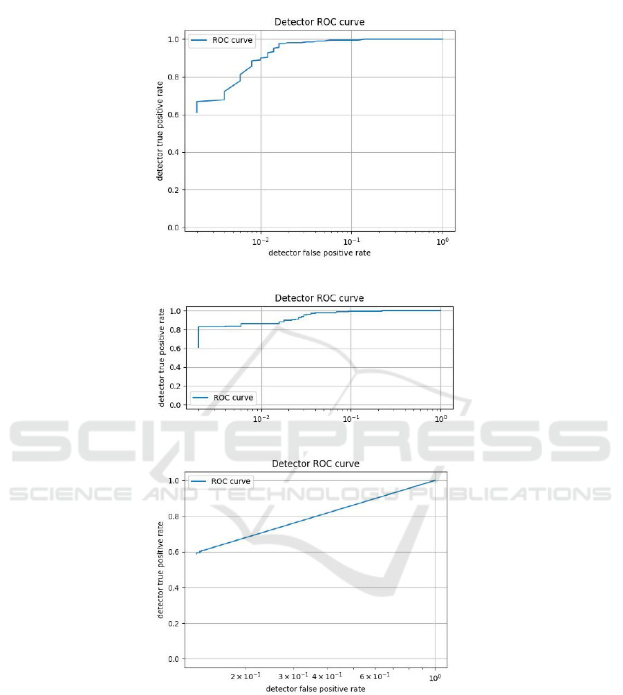
Figure 1: Random forest classiﬁer performance graph.

Figure 2: Logistic regression classiﬁer performance graph.

Figure 3: Naive base classiﬁer performance graph.

the training dataset. The decision of being clean or

suspicious depends on its location compared to the

hyperplane (Chebbi, 2018).

3.5 K-nearest Neighbors Classiﬁer

Having k representing the number of near neighbors,

the idea behind the k-nearest neighbors algorithm is

to consider that if mostly the characteristics of k-

binaries are closest to the characteristics of a binary

that is malicious then the binary is malicious. Else, if

the majority of characteristics of k-binaries are clos-

est to the characteristic of a benign binary, then this

later is benign. For that purpose, the characteristics

and features of the new binary are compared to the

feature of the k samples. When the percentage of

samples in the feature space exceeds a certain num-

ber, then the character (malicious or benign) is de-

Comparing Machine Learning Techniques for Malware Detection

847

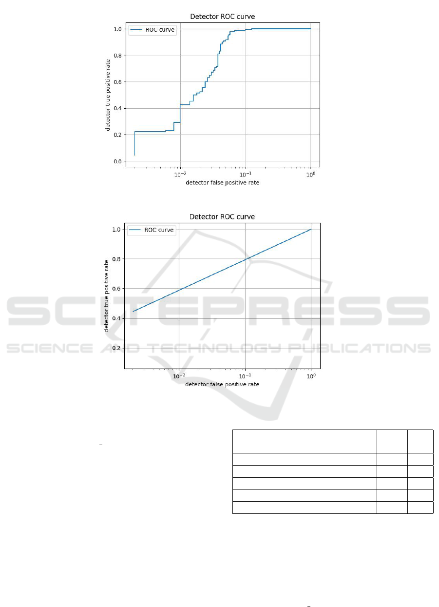
Figure 4: Support vector machines classiﬁer performance graph.

Figure 5: K-nearest neighbors classiﬁer performance graph.

ﬁned. To measure the feature distance (Wang et al.,

2007) between a new binary and the samples in the

training set the euclidean distance function is used to

calculate the shortest distance between two points in

the feature space (Saxe and Sanders, 2018). The K-

Nearest neighbor algorithm is mostly adapted for mal-

ware family classiﬁcation and connect similarities be-

tween binaries.

3.6 Neural Networks

The neural network was divided into layers composed

from an input layer, a middle layer and the output

layer that generates the ﬁnal result. The middle

layer is formed from 512 neurons that uses ReLU

(Rectiﬁed Linear Unit) (Saxe and Sanders, 2018) as

activation function. The last layer uses a sigmoid

function (Gan et al., 2015) and comprise one neuron.

Table 1: Classiﬁers’ Performance.

Classiﬁer FPR TPR

Random forest classiﬁer 10

−2

92%

Logistic regression classiﬁer 10

−2

40%

Naive baise classiﬁer 2.10

−2

65%

Support vector machines classiﬁer 10

−2

40%

k-nearest neighbors classiﬁer 10

−2

59%

Neural network classiﬁer 10

−2

82%

middle = layers.Dense(units=512, activa-

tion=’relu’)(input) output = layers.Dense(units=1,

activation=’sigmoid’)(middle)

Each neuron in the middle layer (dense layer) has

access to all input values. The ReLU activation func-

tion, if positive, will output a positive value, else it is

a zero. The extract features function was applied to

the input (that includes clean and malicious ﬁles) and

ForSE 2020 - 4th International Workshop on FORmal methods for Security Engineering

848

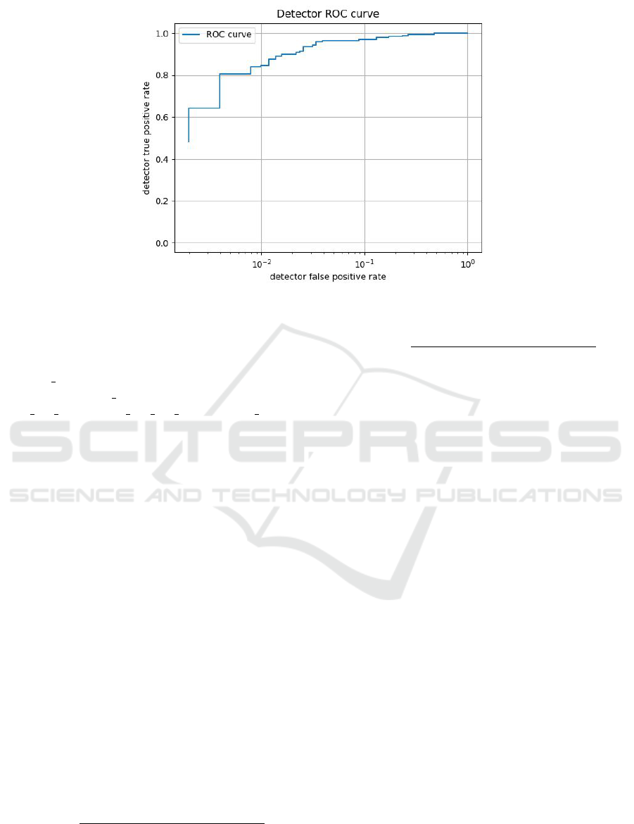
Figure 6: Neural networks classiﬁer performance graph.

then the hash of each token is taken and distributed

among this layer. Furthermore, the training was done

in batches using a feature generator each time.

model.ﬁt generator (

generator=training generator,

steps per epoch=num obs per epoch / batch size,

epochs=10, verbose=1)

4 TECHNICAL ANALYSIS

This section analyses malware leveraging Random

Forest, Logistic Regression, Naive Bayes, Support

Vector Machines, K-nearest neighbors and Neural

Networks algorithms. These models were trained on

datasets from (Saxe and Sanders, 2018). The evalua-

tion between these algorithms includes the Receiver

Operating Characteristic Curve, the detection time

and the limitation of each algorithm.

4.1 Receiver Operating Characteristic

Curve

The Receiver Operating Characteristic Curve (ROC

Curve) permits to predict the correctness of machine

learning algorithms (Bradley, 1997). It consists of a

plot visualizing the algorithm true positive rate (TPR)

versus its false positive rate (FPR).

T PR =

True Positives

True Positives + False Negatives

FPR =

False Positives

False Positives + True Negatives

Predictive rates are divided in four classes:

• True Positive (TP): The binary is correctly pre-

dicted as being malicious.

• True Negative (TN): The binary is correctly pre-

dicted as being benign.

• False Positive (FP): The binary is incorrectly pre-

dicted as being malicious.

• False Negative (FN): The binary is incorrectly

predicted as being benign.

A good classiﬁer will try therefore to maximize

the true positive rate and to minimize the false pos-

itive rate. Comparing the several ROC Curves (Ta-

ble 1), the performance of the random forest classi-

ﬁer is the best among the other algorithms. Besides,

comparing the plots of the detectors, the random for-

est classiﬁer performs well, noting that the execution

can be enhanced when scaling the training dataset to a

bigger amount of test data adding millions of samples.

Others parameters can be added as well.

4.2 Detection Time

To highlight the performance of ML detectors, the

same binaries were tested using the different classi-

ﬁers. Figure 7 summarizes the detection time of each

classiﬁer. For a same new binary to test, the neural

network and logistic regression classiﬁer achieved the

fastest detection rate (4.6 secondes) and the random

forest classiﬁer the slowest average (16.5 secondes).

Comparing Machine Learning Techniques for Malware Detection

849

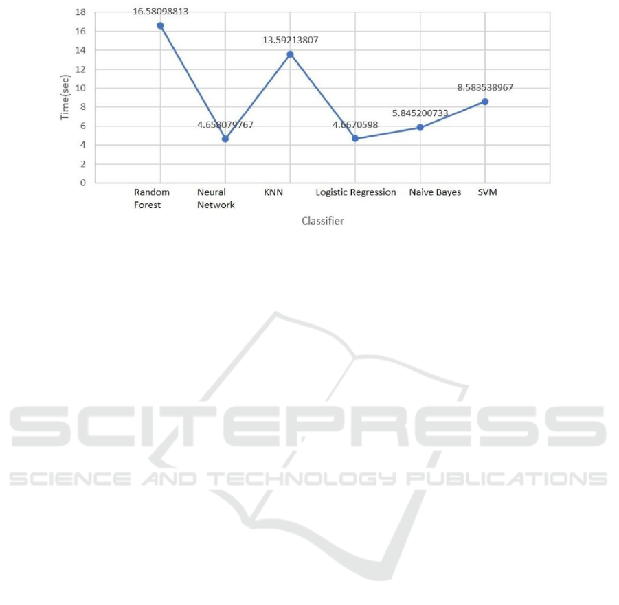
Figure 7: Average Detection Time.

5 CONCLUSION

The information age has recently discovered the value

of big data and information that can hide in dis-

parate, large data sources. The current interest in data

has also spread across multiple applications to detect

and prevent attacks. New technologies permit nowa-

days an advanced analytics approach leveraging big

data. In cybersecurity, machine learning algorithms

can be used to detect external intrusions, for exam-

ple by identifying patterns in the behavior of attack-

ers performing reconnaissance, but also to detect in-

ternal risks. The analysis simply aims to provide vi-

sualization so that human interaction can be applied

to infer ideas. By combining data from system log

ﬁles, historical data on IP addresses, honeypots, sys-

tem and user behaviors, etc. a more comprehensive

overview of a normal situation is conceived. The

wit is to analyze multiple sources and patterns to sig-

nal unwanted behavior. Furthermore, machine learn-

ing is used for attack detection and attribution. Be-

sides, several use cases of machine learning are em-

ployed for penetration testing. The work done in this

paper proves that different approaches can be lever-

aged to detect malware using machine learning. Sev-

eral algorithms have been implemented, trained and

tested. For each algorithm, the methodology of de-

tecting malware have been abridged in details. More-

over, the ROC Curve of each classiﬁer has been il-

lustrated showing that some algorithms perform bet-

ter than others. This study and classiﬁers’ evaluation

show that random forest operates satisfactorily com-

paring to other algorithms even that the average de-

tection time is not the lowest.

Our future plans consist in studying and enhanc-

ing the detection of malware using hybrid training

model and ensemble learning. These algorithms can

be built also leveraging other parameters and training

data. In addition, in a next step we envisage to asso-

ciate multiple analysis techniques to detect malware.

For a complete detection mechanism, we plan to com-

bine static, dynamic and machine learning techniques

to analyse malware.

REFERENCES

Aﬁanian, A., Niksefat, S., Sadeghiyan, B., and Baptiste,

D. (2018). Malware dynamic analysis evasion tech-

niques: A survey. arXiv preprint arXiv:1811.01190.

Boukhtouta, A., Mokhov, S. A., Lakhdari, N.-E., Debbabi,

M., and Paquet, J. (2016). Network malware classi-

ﬁcation comparison using dpi and ﬂow packet head-

ers. Journal of Computer Virology and Hacking Tech-

niques, 12(2):69–100.

Bradley, A. P. (1997). The use of the area under the

roc curve in the evaluation of machine learning algo-

rithms. Pattern recognition, 30(7):1145–1159.

Breiman, L. (2001). Random forests. Machine learning,

45(1):5–32.

Chebbi, C. (2018). Mastering Machine Learning for Pene-

tration Testing. Packt Publishing.

Fan, C.-I., Hsiao, H.-W., Chou, C.-H., and Tseng, Y.-F.

(2015). Malware detection systems based on api log

data mining. In 2015 IEEE 39th annual computer soft-

ware and applications conference, volume 3, pages

255–260. IEEE.

Filiol, E. (2006). Computer viruses: from theory to appli-

cations. Springer Science & Business Media.

Gan, Z., Henao, R., Carlson, D., and Carin, L. (2015).

Learning deep sigmoid belief networks with data aug-

mentation. In Artiﬁcial Intelligence and Statistics,

pages 268–276.

Harrington, P. (2012). Machine learning in action. Manning

Publications Co.

ForSE 2020 - 4th International Workshop on FORmal methods for Security Engineering

850

Hastie, T., Tibshirani, R., Friedman, J., and Franklin, J.

(2005). The elements of statistical learning: data min-

ing, inference and prediction. The Mathematical In-

telligencer, 27(2):83–85.

James, J., Hou, Y., and Li, V. O. (2018). Online false data

injection attack detection with wavelet transform and

deep neural networks. IEEE Transactions on Indus-

trial Informatics, 14(7):3271–3280.

Ligh, M., Adair, S., Hartstein, B., and Richard, M. (2010).

Malware analyst’s cookbook and DVD: tools and

techniques for ﬁghting malicious code. Wiley Pub-

lishing.

Littman, M. L. (1994). Markov games as a framework

for multi-agent reinforcement learning. In Machine

learning proceedings 1994, pages 157–163. Elsevier.

Moor, J. (2003). The Turing test: the elusive standard of

artiﬁcial intelligence, volume 30. Springer Science &

Business Media.

Moubarak, J., Chamoun, M., and Filiol, E. (2017). Compar-

ative study of recent mea malware phylogeny. In 2017

2nd International Conference on Computer and Com-

munication Systems (ICCCS), pages 16–20. IEEE.

Moubarak, J., Chamoun, M., and Filiol, E. (2018). Devel-

oping a k-ary malware using blockchain. In NOMS

2018-2018 IEEE/IFIP Network Operations and Man-

agement Symposium, pages 1–4. IEEE.

Moubarak, J., Chamoun, M., and Filiol, E. (2019). Hiding

malware on distributed storage. In 2019 IEEE Jor-

dan International Joint Conference on Electrical En-

gineering and Information Technology (JEEIT), pages

720–725. IEEE.

Nikolopoulos, S. D. and Polenakis, I. (2017). A graph-

based model for malware detection and classiﬁcation

using system-call groups. Journal of Computer Virol-

ogy and Hacking Techniques, 13(1):29–46.

Quinn, M. J. (2014). Ethics for the information age. Pearson

Boston, MA.

Ruder, S. (2016). An overview of gradient de-

scent optimization algorithms. arXiv preprint

arXiv:1609.04747.

Russell, S. J. and Norvig, P. (2016). Artiﬁcial intelligence: a

modern approach. Malaysia; Pearson Education Lim-

ited,.

Saad, S., Briguglio, W., and Elmiligi, H. (2019). The cu-

rious case of machine learning in malware detection.

arXiv preprint arXiv:1905.07573.

Saxe, J. and Sanders, H. (2018). Malware Data Science. No

Startch Press.

Sikorski, M. and Honig, A. (2012). Practical malware anal-

ysis: the hands-on guide to dissecting malicious soft-

ware. no starch press.

Stoecklin, M. P. (2018). Deeplocker: How ai can power a

stealthy new breed of malware. Security Intelligence,

Wang, J., Neskovic, P., and Cooper, L. N. (2007). Im-

proving nearest neighbor rule with a simple adap-

tive distance measure. Pattern Recognition Letters,

28(2):207–213.

Willems, C., Holz, T., and Freiling, F. (2007). Toward au-

tomated dynamic malware analysis using cwsandbox.

IEEE Security & Privacy, 5(2):32–39.

Wu, S., Wang, P., Li, X., and Zhang, Y. (2016). Effective

detection of android malware based on the usage of

data ﬂow apis and machine learning. Information and

Software Technology, 75:17–25.

Zhu, X., Ghahramani, Z., and Lafferty, J. D. (2003). Semi-

supervised learning using gaussian ﬁelds and har-

monic functions. In Proceedings of the 20th Inter-

national conference on Machine learning (ICML-03),

pages 912–919.

Comparing Machine Learning Techniques for Malware Detection

851