On the Metrics and Adaptation Methods for Domain Divergences of

sEMG-based Gesture Recognition

Istv

an Ketyk

and Ferenc Kov

acs

Nokia Bell Labs, Budapest, Hungary

Keywords:

Machine Learning, Time-series Modeling, sEMG/EMG, Divergence Metrics, Domain Adaptation.

Abstract:

We propose a new metric to measure domain divergence and a new domain adaptation method for time-series

classiﬁcation. The metric belongs to the class of probability distributions-based metrics, is transductive, and

does not assume the presence of source data samples. The 2-stage method utilizes an improved autoregressive,

RNN-based architecture with deep/non-linear transformation. We assess our metric and the performance of our

model in the context of sEMG/EMG-based gesture recognition under inter-session and inter-subject domain

shifts.

1 INTRODUCTION

Machine Learning (ML) is widely used for several

tasks with time-series and biosensor data such as for

human activity recognition, electronic health records

data-based predictions (Ismail Fawaz et al., 2019),

and real-time bionsensor-based decisions. Various

classiﬁcation goals are addressed related to electro-

cardiography (ECG) (Jambukia et al., 2015), elec-

troencephalography (EEG) (Craik et al., 2019; Dose

et al., 2018), and electromyograpy (EMG) (Ketyk

et al., 2019; Hu et al., 2018; Patricia et al., 2014; Du

et al., 2017).

Sensing hand gestures can be done by means of

wearables or by means of image or video analysis of

hand or ﬁnger motion. A wearable-based detection

can physically rely on measuring the acceleration and

rotations of our body parts (arms, hands or ﬁngers)

with Inertial Measurement Unit (IMU) sensors or by

measuring the myo-electric signals generated by the

various muscles of our arms or ﬁngers with EMG sen-

sors. Surface EMG (sEMG) records muscle activity

from the surface of the skin which is above the mus-

cle being evaluated. The signal is collected via sur-

face electrodes.

We are interested in sEMG-sensor placement to

the forearm and performing hand gesture recognition

with ML. In this context, all ML prediction mod-

els suffer from inter-session and inter-subject domain

https://orcid.org/0000-0003-4931-4580

https://orcid.org/0000-0002-9777-0372

domain shift

intra-session

inter-session

inter-subject

Variation in gesture duration,

force level

Variation in sensor placement

Variation in muscle physiology

Figure 1: Domain shift in case of different scenarios.

shifts (see Figure 1).

• Intra Session Scenario: the device is not removed,

and the training and validation data are recorded

together in the same session of the same subject.

In this situation the gesture recognition accuracy

is generally above 90%.

• Inter-session Scenario: the device is reattached,

and the validation data is recorded separately in a

new session of the same subject. Under this do-

main shift the validation accuracy degrades below

50%.

• Inter-subject Scenario: The validation data is on

another subject. In this case, the validation accu-

racy degrades below 50% as well.

Our focus is to investigate: 1) the metrics of these

domain discrepancies, and 2) the adaptation solutions

with special attention on those, which do not rely on

Ketykó, I. and Kovács, F.

On the Metrics and Adaptation Methods for Domain Divergences of sEMG-based Gesture Recognition.

DOI: 10.5220/0009369501210132

In Proceedings of the 13th International Joint Conference on Biomedical Engineering Systems and Technologies (BIOSTEC 2020) - Volume 4: BIOSIGNALS, pages 121-132

ISBN: 978-989-758-398-8; ISSN: 2184-4305

121

source data samples.

This paper is organized as follows, Section 2 pro-

vides a summary of ML, model risks, domains, do-

main divergences, and domain adaptation methods.

Then our source data-absent metric and adaptation

model is introduced in Section 3. Next, we vali-

date our approaches using publicly available sEMG

datasets: the experimental setup and results are de-

scribed in Section 4. Finally, we conclude and sum-

marize our results.

2 RELATED WORK

2.1 Machine Learning

At the most basic level, ML seeks to develop methods

for computers to improve their performance at certain

tasks on the basis of observed data. Almost all ML

tasks can be formulated as making inferences about

missing or latent data from the observed data. To

make inferences about unobserved data from the ob-

served data, the learning system needs to make some

assumptions; taken together these assumptions con-

stitute a model. The probabilistic approach to mod-

eling uses probability theory to express all forms of

uncertainty. Since any sensible model will be un-

certain when predicting unobserved data, uncertainty

plays a fundamental part in modeling. The probabilis-

tic approach to modeling is conceptually very simple:

probability distributions are used to represent all the

uncertain unobserved quantities in a model (including

structural, parametric and noise-related) and how they

relate to the data. Then the basic rules of probabil-

ity theory are used to infer the unobserved quantities

given the observed data. Learning from data occurs

through the transformation of the prior probability

distributions (deﬁned before observing the data), into

posterior distributions (after observing data) (Ghahra-

mani, 2015).

We deﬁne an input space X which is a subset of d-

dimensional real space R

. We deﬁne also a random

variable X with probability distribution P(X) which

takes values drawn from X. We call the realisations

of X feature vectors and noted x

A generative model describes the marginal distri-

bution over X : P

(X), where samples x

of X are ob-

served at learning time in a dataset D and the probabil-

ity distribution depends on some unknown parameter

Θ. A generative model family which is important for

time-series analysis is the autoregressive one. Here,

we ﬁx an ordering of the variables X

,.. .,X

and

the distribution for the i-th random variable depends

on the values of all the preceding random variables

in the chosen ordering X

,.. .,X

i−1

(Bengio et al.,

2015). By the chain rule of probability, we can fac-

torize the joint distribution over the n-dimensions as:

(X) =

∏

i=1

| X

,.. .,X

i−1

) (1)

We deﬁne also an output space Y and a random vari-

able Y taking values y

drawn from Y with distribution

P(Y ). In the supervised learning setting Y is condi-

tioned on X (i.e., Y ∼ P(Y | X )), so the joint distribu-

tion P(X,Y ) is actually P(X)P(Y | X).

A discriminative model is relaxed to the posterior

conditional probability distribution: P

(Y | X) and it

reﬂects straight the discrimination/classiﬁcation task

with lower asymptotic errors than the generative mod-

els. This transductive learning setting has been intro-

duced by Vapnik (Ng and Jordan, 2001).

For all modeling approaches, the learning is to ﬁt

their distributions over the observed variables x

in our

dataset D. With other words (of a statistician), a good

estimate of the unknown parameter Θ would be the

value of Θ that maximizes the likelihood of getting

the data we observed in our dataset D. Formally, the

goal of the Maximum Likelihood Estimation (MLE)

is to ﬁnd the Θ:

Θ = argmax

(D) = argmax

∑

∈D

logP

) (2)

Learning in neural networks is about solving optimi-

sation problems. In case of probabilistic (and differ-

entiable) cost functions, the backpropagation method

(Rumelhart et al., 1986) is an estimator for MLE.

2.2 Risk of Machine Learning Models

We start with the general and probabilistic description

then we move on to the discriminative models.

Let us introduce the concept of loss function. A

loss function L(x

) measures the loss that a model

distribution P

makes on a particular instance x

. Our

goal is to ﬁnd the model P

that minimizes the ex-

pected loss or risk:

R(P

) = E

∼P(X)

[L(x

)] (3)

Note that the loss function which corresponds to MLE

is the log loss −log P

). The risk evaluated on D

is the in-sample error or empirical risk:

R(P

) =

|D|

∑

∈D

L(x

) (4)

The generalization gap is the R(P

) −

R(P

) and

our model intends to have small probability that this

difference is larger than a very small value ε.

BIOSIGNALS 2020 - 13th International Conference on Bio-inspired Systems and Signal Processing

122

In case of supervised learning setting,

we have a paired dataset of observations

D = {(x

),.. .,(x

)}. The loss func-

tion becomes the conditional log-likelihood

L(x

) = −log P

| x

) and the risk is

described as:

R(P

) = E

)∼P(X,Y )

[L(x

)] (5)

Let us introduce the hypothesis space H which is

the set/class of predictors {h : X → Y}. A hypothesis

h estimates the target function f : X → Y from D. The

target function f is a proxy for the conditional distri-

bution P(Y | X ), such as: y

= f (x

) + ζ, where ζ is

the noise term. Substituting h into Equation (5) we

get the transductive version of the risk:

(h) = E

)∼P(X,Y )

[L(y

,h(x

))] (6)

Substituting h into Equation (4):

(h) =

|D|

∑

)∈D

L(y

,h(x

)) (7)

In the transductive setting the generalisation gap can

be quantiﬁed:

Pr[ sup

h∈H

(h) −

(h)| > ε] (8)

2.3 Domain and Domain-shift Concepts

First, it is necessary to clarify what a domain is

and what kind of domain discrepancies there can be.

There are several good survey papers that describe

this ﬁeld deeply e.g., (Kouw, 2018), (Kouw and Loog,

2019), and (Csurka, 2017). In this paper, the do-

main adaptation-related problem statement and nota-

tions follow (Kouw, 2018).

The problem statement is introduced from a clas-

siﬁcation point of view to simplify the deﬁnitions,

but it can be generalized to other supervised machine

learning tasks. A domain contains three elements: In-

put space X, Output space Y and P(X,Y ) joint distri-

bution over X and Y.

Two domains are different if at least one of their

above mentioned components are not equal. In case

of DA the input spaces and output spaces of the do-

mains are the same but the distributions are different.

More general cases belong to different ﬁelds of trans-

fer learning, a detailed taxonomy of transfer learning

tasks can be found in (Pan and Yang, 2010). During

DA there is a trained machine learning model on a

so-called source domain (S) and there is an intent to

apply it on a target domain (T). From this point on-

wards S and T in subscript refer to source and target

domains.

Let us analyze the risk of a source classiﬁer (Equa-

tion (6)) on a target domain T in the cross-domain

setting:

(h) =

∑

y∈Y

L(h(x) | y)P

(x,y)dx

∑

y∈Y

L(h(x) | y)P

(x,y)

dx (9)

It can be seen that the ratio of the source and tar-

get joint distributions (P

(X,Y )/P

(X,Y )) deﬁnes the

risk R

(h). The investigation of this ratio allows us

to deﬁne domain shift cases (Moreno-Torres et al.,

2012): prior shift, covariate shift and concept shift.

In case of prior shift, the marginal distribution of

the labels are different between the source domain and

the target domain P

(Y ) 6= P

(Y ), but the conditional

distributions are equal P

(X | Y ) = P

(X | Y ). Typi-

cal example for prior shift: the symptoms of a disease

are usually population independent but the distribu-

tion of the diseases is population dependent. These

conditions allow us to simplify the risk:

(h) =

∑

y∈Y

L(h(x) | y)P

(x,y)

∑

y∈Y

L(h(x) | y)P

(x,y)

(x | y)P

(y)

(x | y)P

(y)

∑

y∈Y

L(h(x) | y)P

(x,y)

(y)

dx (10)

This means, that the complete labeled dataset from the

target domain is not needed but the estimation of the

marginal distribution of the labels P

(Y ) is needed on

the target domain.

Covariate shift is a well-studied domain shift, for

further reference see (Kouw, 2018). It is deﬁned as

follows: the posterior distributions are equivalent, this

means P

(Y | X) = P

(Y | X), but the marginal distri-

butions of the samples are different P

(X) 6= P

(X).

The typical cause of covariate shift is the sample se-

lection bias. Only the sample distributions determine

the risk:

(h) =

∑

y∈Y

L(h(x) | y)P

(x,y)

∑

y∈Y

L(h(x) | y)P

(x,y)

(y | x)P

(x)

(y | x)P

(x)

∑

y∈Y

L(h(x) | y)P

(x,y)

(x)

dx (11)

In case of concept shift, the marginal distributions

of input vectors are similar on both source and tar-

get domains P

(X) = P

(X), on the other hand, the

On the Metrics and Adaptation Methods for Domain Divergences of sEMG-based Gesture Recognition

123

posterior distributions differ from each other P

(Y |

X) 6= P

(Y | X ). Usually, non-stationary environment

causes this data drift (Widmer and Kubat, 1996). It

is not possible to simplify signiﬁcantly the cross-

domain risk and the DA cannot be done without la-

beled target data:

(h) =

∑

y∈Y

L(h(x) | y)P

(x,y)

∑

y∈Y

L(h(x) | y)P

(x,y)

(y | x)P

(x)

(y | x)P

(x)

∑

y∈Y

L(h(x) | y)P

(x,y)

(y | x)

dx (12)

In general, none of the above mentioned assump-

tions is valid, thus it is not possible to simplify the

risk on target domain. The differing posterior distri-

butions cause the major domain shift related issues.

The optimal transport approach assumes that there is

transport t() that satisﬁes P

(Y | t(X)) = P

(Y | X )

(Courty et al., 2016). Finding this transportation map

is intractable but it is possible to relax it to a sim-

pler optimization problem, where t() is estimated via

a Wasserstein distance minimization between the two

domains (Courty et al., 2016; Kouw and Loog, 2019).

2.4 Divergence Metrics and Theoretical

Bounds

As the input space and output space are common in

case of DA, the distance and divergence metrics of

the distributions can measure and quantify the domain

discrepancies. We elaborate the most common met-

rics in the ﬁeld of DA.

The Kullback-Leibler divergence (Cover and

Thomas, 1991) is a well-known information theory-

based metric between two distributions. It measures

the relative entropy between two distributions. One

of its main disadvantage is, that it is difﬁcult to calcu-

late it from samples in some cases (Ben-David et al.,

2010).

) =

X×Y

(x,y)log



(x,y)



dxdy

∑

y∈Y

(x,y)log



(x,y)



(13)

In general, the KL divergence is an asymmetric met-

ric as D

) 6= D

). A commonly used

symmetric version is the Jensen-Shannon divergence

(Lin, 1991). It measures the total divergence from the

average divergence.

M =

+ P

) =

kM) + D

kM)) (14)

The origin of the Wasserstein distance is the opti-

mal transport problem: a distribution of mass should

be transported to another distribution of mass with

minimal cost. Usually Wassersten-1 distance is used

with the Euclidean distance (Arjovsky et al., 2017).

) = inf

γ∈Π(P

)

(s,t)∼γ

[ks −tk] (15)

where Π(P

) is the set of all joint distributions

with marginals P

and P

. This distance metric al-

lows us to construct a continous and differentiable

loss function (Arjovsky et al., 2017). In case of DA,

this distance is calculated between the marginal dis-

tributions P

(X) and P

(X) to get a tractable problem

(Kouw, 2018).

The H divergence allows to ﬁnd upper bound

to cross-domain risk (Kifer et al., 2004; Ben-David

et al., 2006; Ben-David et al., 2010). The deﬁnitions

and formulas are provided for binary classiﬁcation be-

cause of simpliﬁcation, but they can be generalized to

multi-class problems, as well:

) =

2 sup

h∈H

| Pr

x∼P

(h(x) = 1) − Pr

x∼P

(h(x) = 1)| (16)

(Ben-David et al., 2006) provide two different tech-

niques to estimate H divergence: from ﬁnite sample

and from empirical risk of domain classiﬁer. If the

hypothesis space is symmetrical, the empirical H di-

vergence can be calculated from ﬁnite samples of the

source and target domains:

) =

1−min

h∈H



∑

i=1

I[h(x

S,i

)=1] +

∑

i=1

I[h(x

T,i

)=0]



(17)

where I is an indicator function which gives 1 if pred-

icate is correct, otherwise 0. For the computation of

) during the minimization, the whole hy-

pothesis space H must be tackled. (Ben-David et al.,

2006) introduced an approximation to empirical H di-

vergence, which is called Proxy-A Distance:

) = 2(1 −2

S/T

), (18)

where

S/T

is the empirical risk of a linear domain

classiﬁer, which is trained (in a supervised fashion) to

distinguish the source and target domains.

BIOSIGNALS 2020 - 13th International Conference on Bio-inspired Systems and Signal Processing

124

The cross-domain risk can be estimated by the em-

pirical H divergence:

(h) ≤ R

(h) + R

S+T

∗

) +

) +C(H),

(19)

where C(H) is a complexity measure of hypothesis

space, R

S+T

∗

) is the risk of the so-called single

good hypothesis. The h

∗

is the best classiﬁer that can

generalize on both domains:

S+T

= R

(h) + R

(h)

∗

= argmin

h∈H

S,T

(h)) (20)

The minimization of H divergence gives a better re-

sult, however the the risk of a single good hypothesis

can ruin the performance of the DA. In other words,

if there is no single good hypothesis, the domains are

too far from each other to build an efﬁcient DA.

2.5 Domain Adaptation Techniques

All the adaptive learning strategies focus on identi-

fying how to leverage the information coming from

both the source and target domains. Incorporating ex-

clusively the target domain information is disadvan-

tegous because sometimes there is no labelled targed

data at all, or typically the amount of the labelled tar-

get data is small. Building on information present in

the source domain and adapting that to the target is

generally expected to be the superior solution (Patri-

cia et al., 2014).

We make a split in the viewpoint of source-sample

availability at DA time. We discuss separately meth-

ods that assume source sample availability and meth-

ods that do not, ﬁrst generally, and later in the context

of sEMG-based gesture recognition.

2.5.1 Source Data-based

The majority of the approaches incorporate the unla-

beled source data samples at DA time. Cycle Genera-

tive Adversarial Network (Cycle-GAN) (Zhu et al.,

2017) is a state-of-the-art deep generative model

which is able to learn and implicitly represent the

source and target distributions to pull them close to-

gether in an adversarial fashion. It is composed of two

Generative Adversarial Networks (GANs) (Goodfel-

low et al., 2014) and learns two mappings (A : T → S

and B : S → T ) to achieve the cycle-consistency be-

tween the source and target distributions (A(B(S)) ≈ S

and B(A(T )) ≈ T ) via the minimax game.

Besides the GANs, the autoassociative Auto En-

coder (AE) models are capable of building domain-

invariant representations in their latent space. The

non-linear Denoising AE (DAE) (Glorot et al., 2011)

builds strong representation of the input distribu-

tion with the help of mastering to denoise the in-

put (augmented with noise or corruptions). As a

side effect, the multi-domain input ends up with a

domain-invariant latent representation in the model.

Inspired by the DAE, a linear counterpart: the

Marginalized Denoising AE (mDA) (Chen et al.,

2012) has been proposed to keep the optimization

convex with closed-form solution and achieve orders-

of-magnitude faster computation (at the expense of

the representation power limited to be linear).

Data augmentation with marginalized corruptions

has been studied for the transductive learning set-

ting (Ng and Jordan, 2001) also. The Marginalized

Corrupted Features (MFC) classiﬁer (van der Maaten

et al., 2014) has strong performance in case of valida-

tion under domain shift. In particular, as the corrupt-

ing distribution may be used to shift the data distribu-

tion in the source domain towards the data distribu-

tion in the target domain - potentially, by learning the

parameters of the corrupting distribution using maxi-

mum likelihood.

In the transductive learning setting a classiﬁer can

be explicilty guided to learn a domain-invariant repre-

sentation of the conditional distribution of class labels

P(Y | X ) among two domains. Domain-Adversarial

Neural Network DANN) (Ganin et al., 2016) adver-

sarially connects a binary domain classiﬁer into the

neural network directly exploiting the idea exhibited

by Equation (19).

The binary domain classiﬁer of the DANN (Ganin

et al., 2016) and the mDA (Chen et al., 2012) have

been paired in (Clinchant et al., 2016) to get DA regu-

larization for the linear mDA model. Hence, the mDA

has been explicitly guided to develop a latent rep-

resentation space which is domain-invariant. Linear

classiﬁers built in that latent space have had compara-

ble performance results in several image classiﬁcation

tasks.

The 2-Stage Weighting framework for Multi-

Source Domain Adaptation (2SW-MDA) and the

Geodesic Flow Kernel (GFK) methods in (Patricia

et al., 2014) tackle inter-subject DA for sEMG-based

gesture recognizers. In 2SW-MDA all the data of

each source subject are weighted and combined with

the target subject samples with a linear supervised

method; for GFK the source and target data are em-

bedded in a low-dimensional manifold (with PCA)

and the geodesic ﬂow is used to reduce the domain

shift when evaluating the cross domain sample simi-

larity.

On the Metrics and Adaptation Methods for Domain Divergences of sEMG-based Gesture Recognition

125

2.5.2 Source Data-absent

The overwhelming majority of existing DA methods

makes an assumption of freely available source do-

main data. An equal access to both source and target

data makes it possible to measure the discrepancy be-

tween their distributions and to build representations

common to both target and source domains. In real-

ity, such a simplifying assumption rarely holds, since

source data are routinely a subject of legal and con-

tractual constraints between data owners and data cus-

tomers (Chidlovskii et al., 2016).

Despite the absence of available source samples it

is still possible to rely on: 1) statistical information of

the source retrieved in advance, 2) model(s) trained

on the source data.

CORrelation ALignment (CORAL) (Sun et al.,

2016) minimizes domain shift by aligning the second-

order statistics of source and target distributions,

without requiring any target labels. In contrast to

subspace manifold methods (e.g., (Fernando et al.,

2013)), it aligns the original feature distributions of

the source and target domains, rather than the bases

of lower-dimensional subspaces. CORAL performs

a linear whitening transformation on the source data

then a linear coloring transformation (based on the

second-order statistics of the target data). If the statis-

tical parameters of the source data are retrieved in ad-

vance of the DA then it can be considered as a source

data-absent method.

Adaptive Batch Normalization (AdaBN) (which

is an approximation of the whitening transformation,

usually applied in deep neural networks) is utilised for

DA in (Du et al., 2017) for sEMG-based gesture clas-

siﬁcation. Furthermore, it builds upon the deep Con-

volutional Neural Network (CNN) architecture to ex-

tract spatial information from the high-density sEMG

sensor input. However, it is not modeling the possible

temporal information in the time-series data. Apart

from that, it has state-of-the unsupervised DA perfor-

mance which has been validated under inter-session

and inter-subject domain shifts on several datasets.

(Fernando et al., 2013) introduces (linear) sub-

space alignment between the source and target do-

mains with PCA. In the common linear subspace clas-

siﬁers can be trained with comparable performance.

The alignments (i.e., the PCA transformations) are

learned on the source and target data, respectively.

If the source alignment is learned (as a model of the

source) in advance of the DA then it can be considered

as a source data-absent method.

(Farshchian et al., 2019) introduces the Adversar-

ial Domain Adaptation Network (ADAN) with an AE

(trained on the source data) for Brain-Machine Inter-

faces (BMIs). With the representation power of the

AE it is possible to capture the source distribution

then continously align the shifting target distributions

back to it. ADAN is trained in an adversarial fashion

with an Energy-based GAN architecture (Zhao et al.,

2017) where the ”energy” is the reconstruction loss of

the AE, and the domain shifts are represented as the

residual-loss distributions of the AE. ADAN learns

via the minimax game to pull the target residual dis-

tributions to those of the source.

In the transductive learning setting (Ng and Jor-

dan, 2001) there are several source data-absent DA

approaches building on the pre-trained source classi-

ﬁer(s).

The Transductive Doman Adaptation (TDA) in

(Chidlovskii et al., 2016) utilizes the representation

capabilities of the mDA (Chen et al., 2012) to (lin-

early) adapt the output of a trained source classiﬁer to

the target domain. TDA performs unsupervised DA in

closed form without the presence of any extra source

information.

The transductive Multi-Adapt and the Multi-

Kernel Adaptive Learning (MKAL) in (Patricia et al.,

2014) both tackle the inter-subject DA for sEMG-

based gesture recognizers by the adaptation of trained

source classiﬁers. In Multi-Adapt, an SVM is learned

from each source and used as reference (resulted by

a convex optimization) when performing supervised

learning on the target dataset. In MKAL each SVM

source classiﬁer predicts on the target samples and the

scores are used as extra input features for the learning

of the gesture classiﬁer on the target dataset. Multi-

Adapt and MKAL have had comparable performance

at that time even though these models do not capture

the available temporal information in the time-series

data.

(Dose et al., 2018) builds a BMI and investigates

DA for multi-variate EEG time-series data classiﬁ-

cation. The time-series classiﬁcation of the multi-

variate EEG signals is a very similar challenge to the

multi-variate sEMG signals. (Dose et al., 2018) cap-

tures both the spatial and temporal correlations in the

data with a CNN architecture. However, the DA is

about supervised ﬁne-tuning of all the model parame-

ters on the target subject which is suboptimal as high-

lighted by (Du et al., 2017; Ketyk

o et al., 2019).

The 2-Stage Recurrent Neural Network (2SRNN)

model for sEMG gesture recognition and DA in

(Ketyk

o et al., 2019) can be viewed as the deep neu-

ral, autoregressive modeling analogy of the MKAL

(Patricia et al., 2014). It utilizes a trained source clas-

siﬁer and performs supervised DA to the target (ses-

sion or subject) via learning a linear transformation

between the domains. The transformation is then ap-

BIOSIGNALS 2020 - 13th International Conference on Bio-inspired Systems and Signal Processing

126

𝑥

𝑡

𝑥

…

ℎ

𝑡

𝑥

𝒕

ℎ

𝟐

ℎ

𝟏

ℎ

𝑡

ℎ

𝟎

Figure 2: RNN in compact and unrolled representations.

plied to the input (samples coming from the target).

Learning is on the divergent (inter-session or inter-

subject) domains via the backpropagation (Rumelhart

et al., 1986) of the classiﬁer’s cross-entropy loss to its

DA layer (which is a linear readout layer of the input).

The size of its DA layer is less than 1% of the over-

all 2SRNN (in terms of the trainable parameters) so it

achieves fast computation of the DA, and the 2SRNN

has the state-of-the-art performance in inter-session

and inter-subject domain shift validations.

3 OUR DIVERGENCE METRIC

AND ADAPTATION METHOD

We provide a sequential, source data-absent, trans-

ductive, probability-based divergence metric and DA

method as well. First, we introduce the RNN archi-

tecture for temporal modeling, then the source data-

absent and transductive 2SRNN model in details.

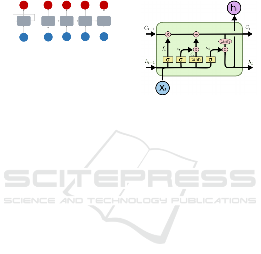
3.1 Recurrent Neural Network

Recurrent Neural Network (RNN) (Jordan, 1986)

is an autoregressive neural network architecture in

which there are feedback loops in the system. Feed-

back loops allow processing the previous output with

the current input, thus making the network stateful,

being inﬂuenced by the earlier inputs in each step (see

Figure 2). A hidden layer that has feedback loops is

also called a recurrent layer. The mathematical rep-

resentation of a simple recurrent layer can be seen in

Equation (21):

= σ

+ W

t−1

+ b

)

= σ

+ b

)

(21)

The hidden state h

depends on the input x

and

the previous hidden state h

t−1

. There is a non-linear

dependency (via the σ() wrapper) between them.

However, regular RNNs suffer from the vanish-

ing or exploding gradient problems which means that

the gradient of the loss function decays/rises expo-

nentially with time, making it difﬁcult to learn long-

term temporal dependencies in the input data (Pas-

canu et al., 2013). Long Short Term Memory (LSTM)

Figure 3: LSTM cell architecture (Olah, 2015).

recurrent cells have been proposed to solve these

(Hochreiter and Schmidhuber, 1997).

= σ(W

· [h

t−1

] + b

)

= σ(W

· [h

t−1

] + b

)

= tanh(W

· [h

t−1

] + b

)

= f

∗ C

t−1

+ i

∗

= σ(W

· [h

t−1

] + b

)

= o

∗ tanh(C

)

(22)

LSTM units contain a set of (learnable) gates that are

used to control the stages when information enters the

cell (input gate: i

), when it is output (output gate:

) and when it is forgotten (forget gate: f

) as seen

in Equation (22). This architecture allows the neural

network to learn longer-term dependencies because it

learn also how to incorporate an additional informa-

tion channel C

. In Figure 3 yellow rectangles rep-

resent a neural network layer, circles are point-wise

operations and arrows denote the ﬂow of data. Lines

merging denote concatenation (notation of [] in Equa-

tion (22)), while a line forking denote its content be-

ing copied and the copies going to different locations.

For autoregressive modeling of time-series data,

RNN with LSTM cells is widely adopted (Hu et al.,

2018; Ketyk

o et al., 2019).

3.2 2-Stage Recurrent Neural

Network-based Domain Divergence

Metric

Similarly to ADAN (Farshchian et al., 2019), we build

a source data-absent, probability-based divergence

metric on the validation loss of the source model to

measure domain shifts. In ADAN, the distribution of

the residual loss (of the AE) is incorporated to express

On the Metrics and Adaptation Methods for Domain Divergences of sEMG-based Gesture Recognition

127

𝑥

𝑡

′

𝑥

′

𝑥

′

𝑥

′

…

ℎ

𝑡

𝒢-softmax

LSTM

𝑥

𝒕

𝑥

𝒕

′

Figure 4: The 2SRNN architecture: 1) DA component,

2) Sequence classiﬁer.

the divergence of target distributions from the one of

source. However, we follow the transductive learn-

ing setting and directly take the (cross-entropy) loss

of the source classiﬁer (exhibiting Equation (5)). Our

source classiﬁer is a sequential model (i.e., built on

the autoregressive RNN architecture to have temporal

modeling capabilites). For this task, we utilise the se-

quence classiﬁer of the 2SRNN architecture (Ketyk

et al., 2019).

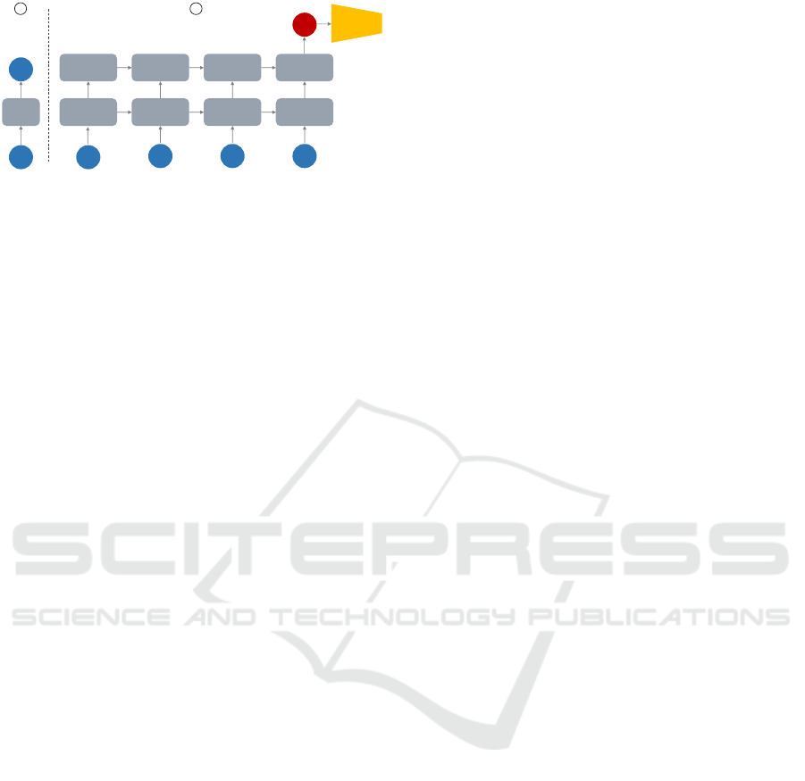
The sequence classiﬁer of 2SRNN (visualised as

block 2 in Figure 4) is a deep stacked RNN with

the many-to-one setup followed by a G-way fully-

connected layer (G is the number of gestures to be

recognized) and a softmax transformation at the out-

put. The sequence classiﬁer is directly modeling the

conditional distribution of P(Y | X), where Y belongs

to a categorical distribution with G (gesture) classes.

Learning is via the categorical cross-entropy loss (of

the ground truth and the predicted Y ):

cross-entropy

= −

∑

g∈G

logP

Θ,g

, (23)

where I

is the indicator function whether class label

g is the correct classiﬁcation for the given observation

and P

Θ,g

is the predicted probability that the observa-

tion is of class g.

For the divergence measure of distributions (be-

tween the source and target domains), we take the

categorical cross-entropy losses of the sequence clas-

siﬁer in the following way: the classiﬁer is trained on

the source distribution then evaluated on a target one.

Hence, the resulting L

cross-entropy

expresses the domain

shift in the loss space of the two domains. The cross-

entropy between P

and P

H(P

) = H(P

) + D

(S||T ). (24)

The L

cross-entropy

expresses the empirical H(P

) by

the model. A valid source classiﬁer is expected to

model the source with the entropy of H(P

) ≈ 1/G, so

in fact the cross-entropy H(P

) captures the actual

Kullback-Leibler divergence among P

and P

(Equa-

tion (13)).

Furthermore, let µ

and µ

be the corresponding

means of P

and P

. We measure the dissimilarity be-

tween these two distributions by a lower bound to the

Wasserstein distance (Equation (15)), provided by the

absolute value of the difference between the means

(Berthelot et al., 2017):

) ≥ |µ

− µ

|. (25)

The difference of the empirical means with the

cross-entropy

approximates Equation (25).

3.3 2-Stage Recurrent Neural

Network-based Domain Adaptation

We build a source data-absent, probability distribution

of L

cross-entropy

-driven DA. (Ketyk

o et al., 2019) imple-

ments a linear version (L-2SRNN), we extend it to a

deep, non-linear one, and name it the Deep 2SRNN

(D-2SRNN). Generally, the DA is applied to the input

of the sequence classiﬁer at each timestamp t (visu-

alised as block 1 in Figure 4). L-2SRNN learns the

weights of a linear transformation:

= Mx

+ b. (26)

D-2SRNN learns the weights of chained non-linear

transformations:

= σ(M

· σ(M

+ b

) + b

). (27)

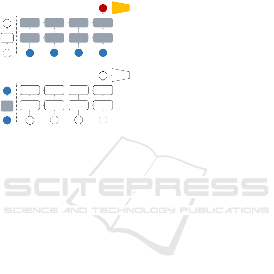
Figure 5 presents the two consecutive stages of the

DA process:

I) The DA component initially is the identity trans-

formation, and the weights of it are frozen. The

sequence classiﬁer is trained from scratch on the

labelled source dataset.

II) The weights of the sequence classiﬁer are frozen

and the DA component’s weights are trained on

a minor subset of the labelled target dataset:

cross-entropy

is backpropagated (Rumelhart et al.,

1986) to the DA component during the process.

Hence, the D

||P

) in Equation (24) or ex-

pressed via the D

) in Equation (25) gets

minimized.

4 RESULTS

We perform experiments to validate our divergence

metric and DA for sEMG-based gesture recognition in

case of inter-session and inter-subject scenarios. We

follow the exact same hyperparametrization and net-

work implementations as in (Ketyk

o et al., 2019). The

parameters M,M

∈ R

f × f

in Equations (26) and

BIOSIGNALS 2020 - 13th International Conference on Bio-inspired Systems and Signal Processing

128

𝑥

𝑡

′

𝑥

′

𝑥

′

𝑥

′

…

ℎ

𝑡

𝒢-softmax

LSTM

…

𝑥

𝒕

𝑥

𝒕

′

trained

fixed

Stage I.: source classifier pre-training

fixed

trained

Stage II.: target domain adaptation

Figure 5: The 2SRNN method: I) Source classiﬁer pre-

training, II) Domain adaptation.

(27), where f is equal to the size of the input features

(number of sEMG channels). The σ() non-linearity in

Equation (27) is the REctiﬁed Linear Unit (Nair and

Hinton, 2010).

For the sequence classiﬁer we use a 2-stack RNN

with LSTM cells. Each LSTM cell has a dropout

with the probability of 0.5 and 512 hidden units. The

RNN is followed by a G-way fully-connected layer

with 512 units (dropout with a probability of 0.5) and

a softmax classiﬁer. Adam (Kingma and Ba, 2014)

with the learning rate of 0.001 is used for the stochas-

tic gradient descent optimization. The size of the

DA component in both the linear and deep cases is

less than 1% of the total trainable network parame-

ters. The gesture recognition accuracy is calculated

as given below:

Classiﬁcation Accuracy =

Correct

Total

∗ 100% (28)

We investigate the inter-session and inter-subject

divergences and validate our DA method on public

sparse and dense sEMG datasets. We follow the ex-

periment setups of previous works for comparabil-

ity. Since we do sequential modeling in all experi-

ments, we decompose the sEMG signals into small se-

quences using the sliding window strategy with over-

lapped windowing scheme. The sequence length must

be shorter than 300 ms to satisfy real-time usage con-

straints. To compare our current experiments with

previous works, we follow the segmentation strategy

in previous studies.

The dense-electrode sEMG CapgMyo dataset has

been thoroughly analysed by (Du et al., 2017; Hu

et al., 2018; Ketyk

o et al., 2019) such as the sparse-

electrode sEMG NinaPro dataset by (Patricia et al.,

2014; Du et al., 2017; Ketyk

o et al., 2019).

The CapgMyo dataset (Du et al., 2017): includes

HD-sEMG data for 128 electrode channels. The sam-

pling rate is 1 KHz:

1. DB-b: 8 isometric, isotonic hand gestures from

10 subjects in two recording sessions on different

days.

2. DB-c: 12 basic movements of the ﬁngers were ob-

tained from 10 subjects.

We downloaded the pre-processed version from http:

//zju-capg.org/myo/data to work with the exact same

data as (Du et al., 2017; Ketyk

o et al., 2019) for fair

comparison. In that version, the power-line interfer-

ence was removed from the sEMG signals by using

a band-stop ﬁlter (45–55 Hz, second-order Butter-

worth). Only the static part of the movements was

kept in it (for each trial, the middle one-second win-

dow, 1000 frames of data). They used the middle,

one-second data to ensure that no transition move-

ments are included in it. We rescaled the data to have

zero mean and unit variance, then we rectiﬁed it and

applied smoothing (as low-pass ﬁltering).

The NinaPro DB-1 dataset (Patricia et al., 2014)

contains sparse 10-channel sEMG recordings:

1. Gesture numbers 1–12: 12 basic movements of

the ﬁngers (ﬂexions and extensions). These are

equivalent to gestures in CapgMyo DB-c.

The data is recorded at a sampling rate of 100 Hz, us-

ing 10 sparsely located electrodes placed on subjects’

upper forearms. The sEMG signals were rectiﬁed

and smoothed by the acquisition device. We down-

loaded the version from http://zju-capg.org/myo/data/

ninapro-db1.zip to use the exact same data as (Du

et al., 2017; Ketyk

o et al., 2019) for fair comparison.

For each trial, we used the middle 1.5-second win-

dow, 180 frames of data to get the static part of the

gestures.

4.1 Divergence Metric Validation

We validate the proposed domain divergence metric

in Section 3.2 on the CapgMyo DB-b dataset which

covers both the inter-session and inter-subject scenar-

ios.

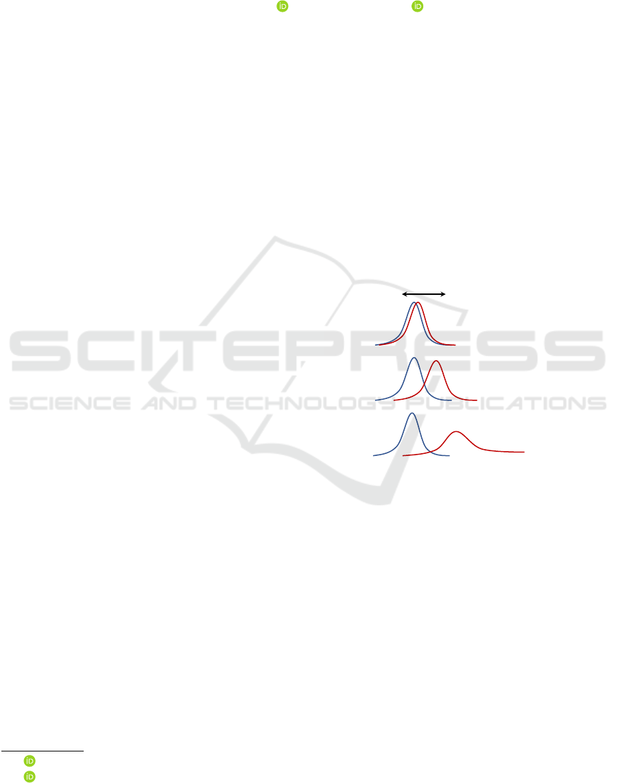
The divergence results are shown in Figure 6 and

Figure 7. In both ﬁgures the empirical distributions

of L

cross-entropy

are illustrated by their histograms and

mean values.

Figure 6 presents the inter-session and inter-

subject divergences before DA. The values with red

(µ

,µ

) represent the means of L

cross-entropy

; µ

On the Metrics and Adaptation Methods for Domain Divergences of sEMG-based Gesture Recognition

129

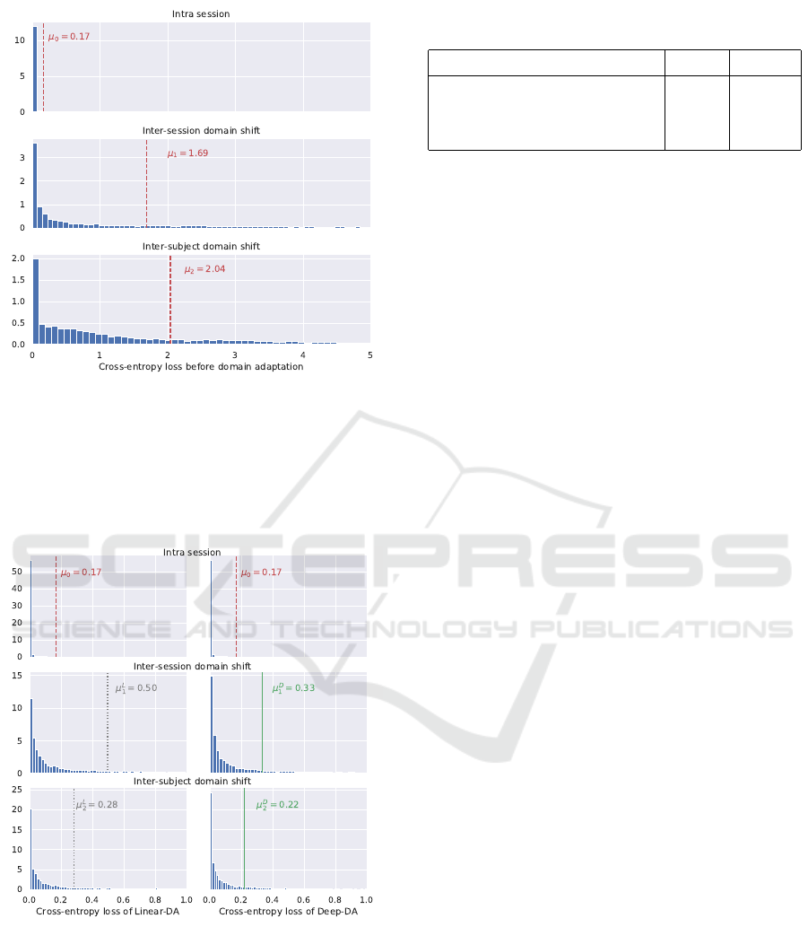
Figure 6: Histograms and mean values in case of the dif-

ferent domain shifts: histograms represent the distributions

cross-entropy loss of the classiﬁer on validation data before

domain adaptation. The values with red (µ

,µ

) repre-

sent the means of validation loss; µ

is the low mean loss in

case of intra session; µ

and µ

(along with their histograms)

show high inter-session and inter-subject distribution diver-

gences.

Figure 7: Histograms and mean values in case of different

domain shifts and adaptation solutions: histograms repre-

sent the distributions of cross-entropy loss of the classiﬁer

on validation data after domain adaptation. Intra session

statistics (µ

) represent the source distribution (towards the

divergent distributions are aimed to be adapted). The his-

tograms and corresponding mean values with gray (µ

,µ

)

represent the validation loss after linear domain adapta-

tion; the histograms and corresponding mean values with

green (µ

,µ

) represent the validation loss after deep do-

main adaptation.

Table 1: Inter-session recognition accuracy results on

CapgMyo DB-b.

pre-DA post-DA

AdaBN (Du et al., 2017) 47.9% 63.3%

L-2SRNN (Ketyk

o et al., 2019) 54.6% 83.8%

D-2SRNN 54.6% 85.9%

the low mean loss in case of intra session; µ

and µ

(along with their histograms) show high inter-session

and inter-subject domain shifts. µ

shows the power

of the sequence classiﬁer: µ

= 0.17 is close to the

theoretical lower bound of cross-entropy which is

H(S) = 0.125 in the current case.

Figure 7 presents the inter-session and inter-

subject divergences after DA. Intra session statistics

(µ

) represent the source distribution (towards the di-

vergent distributions are aimed to be adapted). The

histograms and corresponding mean values with gray

(µ

,µ

) represent the validation loss after L-2SRNN

DA; the histograms and corresponding mean values

with green (µ

,µ

) represent the validation loss after

D-2SRNN DA. In all cases, the post-DA L

cross-entropy

distributions appear to be close to one of the source.

4.2 Domain Adaptation Validation

For comparison purposes, we take the exact same

pre-trained source classiﬁers from (Ketyk

o et al.,

2019) and perform D-2SRNN DA (described in Sec-

tion 3.3). The evaluation of the D-2SRNN DA is ex-

actly the same as of the L-2SRNN and the AdaBN

(Du et al., 2017) approaches. Furthermore, the com-

parison to the MKAL (Patricia et al., 2014) also is

exactly the same as in (Du et al., 2017; Ketyk

o et al.,

2019).

Table 1 presents the inter-session recognition ac-

curacy results on the dense CapgMyo DB-b dataset.

The L-2SRNN and D-2SRNN share the exact same

pre-trained source classiﬁer models. The D-2SRNN

DA brings 57.3% improvement which is better by 2.1

percentage points than the L-2SRNN.

Table 2 shows the inter-subject recognition ac-

curacy results on the dense CapgMyo DB-b & DB-

c and the sparse NinaPro DB-1 datasets. The L-

2SRNN and D-2SRNN share the exact same pre-

trained source classiﬁer models. The D-2SRNN DA

achieves: 74.9% improvement on the DB-b, 156.3%

improvement on the DB-c, 107.4% improvement on

the DB-1. The performance ratio (between the deep

and the linear solutions) is 3.4% in case of the dense

datasets, and 11.7% in case of the sparse one which

suggests that there is higher gain by non-linear adap-

tation in case of a sparse-electrode situation.

BIOSIGNALS 2020 - 13th International Conference on Bio-inspired Systems and Signal Processing

130

Table 2: Inter-subject recognition accuracy results on dense CapgMyo and sparse NinaPro datasets.

pre-DA post-DA

DB-b DB-c DB-1 DB-b DB-c DB-1

AdaBN (Du et al., 2017) 39.0% 26.3% - 55.3% 35.1% -

MKAL (Patricia et al., 2014) - - 30% - - 55%

L-2SRNN (Ketyk

o et al., 2019) 52.6% 34.8% 35.1% 89.9% 85.4% 65.2%

D-2SRNN 52.6% 34.8% 35.1% 92.0% 89.2% 72.8%

5 CONCLUSIONS

We showed that the divergences between the em-

pirical distributions of the cross-entropy losses by a

source classiﬁer trained on the source distribution and

evaluated on the target one is a valid measure for the

domain shifts between source and target. It works

in the absence of source data and a domain adapta-

tion method built on minimizing that divergence is

an effective solution in the transductive learning set-

ting. Furthermore, we pointed out that this metric

and the corresponding adaptation method is applica-

ble to investigate and improve sEMG-based gesture

recognition performance in inter-session and inter-

subject scenarios under severe domain shifts. The

proposed deep/non-linear transformation component

enhances the performance of the 2SRNN architecture

especially in a sparse sEMG setting.

The code is available at https://github.com/ketyi/

Deep-2SRNN.

ACKNOWLEDGEMENTS

Project no. FIEK 16-1-2016-0007 has been imple-

mented with the support provided of the National Re-

search, Development and Innovation Fund of Hun-

gary, ﬁnanced under the FIEK 16 funding scheme.

REFERENCES

Arjovsky, M., Chintala, S., and Bottou, L. (2017). Wasser-

stein generative adversarial networks. In Proceed-

ings of the 34th International Conference on Machine

Learning, volume 70, pages 214–223.

Ben-David, S., Blitzer, J., Crammer, K., Kulesza, A.,

Pereira, F., and Vaughan, J. W. (2010). A theory of

learning from different domains. Machine Learning,

79(1):151–175.

Ben-David, S., Blitzer, J., Crammer, K., and Pereira, F.

(2006). Analysis of representations for domain adap-

tation. In Proceedings of the 19th International Con-

ference on Neural Information Processing Systems,

NIPS’06, pages 137–144, Cambridge, MA, USA.

MIT Press.

Bengio, S., Vinyals, O., Jaitly, N., and Shazeer, N. (2015).

Scheduled sampling for sequence prediction with re-

current neural networks. In Cortes, C., Lawrence,

N. D., Lee, D. D., Sugiyama, M., and Garnett, R., edi-

tors, Advances in Neural Information Processing Sys-

tems 28, pages 1171–1179. Curran Associates, Inc.

Berthelot, D., Schumm, T., and Metz, L. (2017). BE-

GAN: Boundary Equilibrium Generative Adversarial

Networks. ArXiv, abs/1703.10717.

Chen, M., Xu, Z., Weinberger, K. Q., and Sha, F.

(2012). Marginalized denoising autoencoders for do-

main adaptation. In Proceedings of the 29th Interna-

tional Coference on International Conference on Ma-

chine Learning, ICML’12, pages 1627–1634, USA.

Omnipress.

Chidlovskii, B., Clinchant, S., and Csurka, G. (2016). Do-

main adaptation in the absence of source domain data.

In Proceedings of the 22Nd ACM SIGKDD Interna-

tional Conference on Knowledge Discovery and Data

Mining, KDD ’16, pages 451–460, New York, NY,

USA. ACM.

Clinchant, S., Csurka, G., and Chidlovskii, B. (2016). A do-

main adaptation regularization for denoising autoen-

coders. In Proceedings of the 54th Annual Meeting

of the Association for Computational Linguistics (Vol-

ume 2: Short Papers), pages 26–31, Berlin, Germany.

Association for Computational Linguistics.

Courty, N., Flamary, R., Tuia, D., and Rakotomamonjy,

A. (2016). Optimal transport for domain adaptation.

IEEE Transactions on Pattern Analysis and Machine

Intelligence, 39(9):1853–1865.

Cover, T. M. and Thomas, J. A. (1991). Elements of Infor-

mation Theory. Wiley-Interscience, New York, NY,

USA.

Craik, A., He, Y., and Contreras-Vidal, J. L. (2019). Deep

learning for electroencephalogram (EEG) classiﬁca-

tion tasks: a review. Journal of Neural Engineering,

16(3):031001.

Csurka, G. (2017). Domain adaptation for visual

On the Metrics and Adaptation Methods for Domain Divergences of sEMG-based Gesture Recognition

131

applications: A comprehensive survey. CoRR,

abs/1702.05374.

Dose, H., Møller, J. S., Iversen, H. K., and Puthusserypady,

S. (2018). An end-to-end deep learning approach to

MI-EEG signal classiﬁcation for BCIs. Expert Sys-

tems with Applications, 114:532 – 542.

Du, Y., Jin, W., Wei, W., Hu, Y., and Geng, W. (2017). Sur-

face EMG-based inter-session gesture recognition en-

hanced by deep domain adaptation. Sensors (Basel,

Switzerland), 17(3):458. 28245586[pmid].

Farshchian, A., Gallego, J. A., Cohen, J. P., Bengio, Y.,

Miller, L. E., and Solla, S. A. (2019). Adversarial do-

main adaptation for stable brain-machine interfaces.

In International Conference on Learning Representa-

tions.

Fernando, B., Habrard, A., Sebban, M., and Tuytelaars, T.

(2013). Unsupervised visual domain adaptation using

subspace alignment. In ICCV.

Ganin, Y., Ustinova, E., Ajakan, H., Germain, P.,

Larochelle, H., Laviolette, F., Marchand, M., and

Lempitsky, V. (2016). Domain-adversarial training of

neural networks. J. Mach. Learn. Res., 17(1):2096–

2030.

Ghahramani, Z. (2015). Probabilistic machine learning and

artiﬁcial intelligence. Nature, 521(7553):452–459.

Glorot, X., Bordes, A., and Bengio, Y. (2011). Domain

adaptation for large-scale sentiment classiﬁcation: A

deep learning approach. In Getoor, L. and Scheffer,

T., editors, ICML, pages 513–520. Omnipress.

Goodfellow, I., Pouget-Abadie, J., Mirza, M., Xu, B.,

Warde-Farley, D., Ozair, S., Courville, A., and Ben-

gio, Y. (2014). Generative Adversarial Nets. In Ad-

vances in Neural Information Processing Systems 27.

Hochreiter, S. and Schmidhuber, J. (1997). Long Short-

Term Memory. Neural Comput., 9(8):1735–1780.

Hu, Y., Wong, Y., Wei, W., Du, Y., Kankanhalli, M.,

and Geng, W. (2018). A novel attention-based hy-

brid CNN-RNN architecture for sEMG-based gesture

recognition. PLOS ONE, 13(10):1–18.

Ismail Fawaz, H., Forestier, G., Weber, J., Idoumghar, L.,

and Muller, P.-A. (2019). Deep learning for time series

classiﬁcation: a review. Data Mining and Knowledge

Discovery, 33(4):917–963.

Jambukia, S. H., Dabhi, V. K., and Prajapati, H. B. (2015).

Classiﬁcation of ECG signals using machine learning

techniques: A survey. In 2015 International Confer-

ence on Advances in Computer Engineering and Ap-

plications, pages 714–721.

Jordan, M. I. (1986). Attractor dynamics and parallelism

in a connectionist sequential machine. In Proceedings

of the Eighth Annual Conference of the Cognitive Sci-

ence Society, pages 531–546. Hillsdale, NJ: Erlbaum.

Ketyk

o, I., Kov

acs, F., and Varga, K. Z. (2019). Domain

adaptation for sEMG-based gesture recognition with

Recurrent Neural Networks. In 2019 International

Joint Conference on Neural Networks (IJCNN), pages

1–7.

Kifer, D., Ben-David, S., and Gehrke, J. (2004). Detecting

change in data streams. In Proceedings of the Thirtieth

International Conference on Very Large Data Bases -

Volume 30, VLDB ’04, pages 180–191. VLDB En-

dowment.

Kingma, D. P. and Ba, J. (2014). (adam): A

method for stochastic optimization. cite

arxiv:1412.6980Comment: Published as a con-

ference paper at the 3rd International Conference for

Learning Representations, San Diego, 2015.

Kouw, W. M. (2018). An introduction to domain adaptation

and transfer learning. CoRR, abs/1812.11806.

Kouw, W. M. and Loog, M. (2019). A review of

single-source unsupervised domain adaptation. CoRR,

abs/1901.05335.

Lin, J. (1991). Divergence measures based on the shannon

entropy. IEEE Transactions on Information Theory,

37(1):145–151.

Moreno-Torres, J. G., Raeder, T., Alaiz-Rodr

ıGuez, R.,

Chawla, N. V., and Herrera, F. (2012). A unify-

ing view on dataset shift in classiﬁcation. Pattern

Recogn., 45(1):521–530.

Nair, V. and Hinton, G. E. (2010). Rectiﬁed linear units im-

prove restricted boltzmann machines. In Proceedings

of ICML’10, pages 807–814, USA.

Ng, A. Y. and Jordan, M. I. (2001). On discriminative

vs. generative classiﬁers: A comparison of logistic

regression and naive bayes. In Proceedings of the

14th International Conference on Neural Information

Processing Systems: Natural and Synthetic, NIPS’01,

pages 841–848, Cambridge, MA, USA. MIT Press.

Olah, C. (2015). Understanding LSTM Networks.

Pan, S. J. and Yang, Q. (2010). A survey on transfer learn-

ing. IEEE Transactions on Knowledge and Data En-

gineering, 22(10):1345–1359.

Pascanu, R., Mikolov, T., and Bengio, Y. (2013). On the dif-

ﬁculty of training recurrent neural networks. In Pro-

ceedings of ICML’13.

Patricia, N., Tommasi, T., and Caputo, B. (2014). Multi-

source Adaptive Learning for Fast Control of Pros-

thetics Hand. In Proceedings of the 22nd Inter-

national Conference on Pattern Recognition, pages

2769–2774. IEEE.

Rumelhart, D. E., Hinton, G. E., and Williams, R. J. (1986).

Parallel distributed processing: Explorations in the

microstructure of cognition, vol. 1. chapter Learning

Internal Representations by Error Propagation, pages

318–362. MIT Press, Cambridge, MA, USA.

Sun, B., Feng, J., and Saenko, K. (2016). Return of frustrat-

ingly easy domain adaptation. In AAAI.

van der Maaten, L., Chen, M., Tyree, S., and Wein-

berger, K. Q. (2014). Marginalizing corrupted fea-

tures. CoRR, abs/1402.7001.

Widmer, G. and Kubat, M. (1996). Learning in the presence

of concept drift and hidden contexts. Mach. Learn.,

23(1):69–101.

Zhao, J., Mathieu, M., and LeCun, Y. (2017). Energy-based

generative adversarial networks. ICLR 2017.

Zhu, J., Park, T., Isola, P., and Efros, A. A. (2017). Unpaired

image-to-image translation using cycle-consistent ad-

versarial networks. In 2017 IEEE International Con-

ference on Computer Vision (ICCV), pages 2242–

2251.

BIOSIGNALS 2020 - 13th International Conference on Bio-inspired Systems and Signal Processing

132