3D Model-based 6D Object Pose Tracking on RGB Images using Particle

Filtering and Heuristic Optimization

Mateusz Majcher and Bogdan Kwolek

AGH University of Science and Technology, 30 Mickiewicza, 30-059 Krakow, Poland

Keywords:

6D Object Pose Tracking, Region-based Pose Estimation, Image Segmentation, Optimization.

Abstract:

We present algorithm for tracking 6D pose of the object in a sequence of RGB images. The images are acquired

by a calibrated camera. The object of interest is segmented by an U-Net neural network. The network is trained

in advance to segment a set of objects from the background. The 6D pose of the object is estimated through

projecting the 3D model to image and then matching the rendered object with the segmented object. The

objective function is calculated using object silhouette and edge scores determined on the basis of distance

transform. A particle ﬁlter is used to estimate the posterior probability distribution. A k-means++ algorithm,

which applies a sequentially random selection strategy according to a squared distance from the closest center

already selected is executed on particles representing multi-modal probability distribution. A particle swarm

optimization is then used to ﬁnd the modes in the probability distribution. Results achieved by the proposed

algorithm were compared with results obtained by a particle ﬁlter and a particle swarm optimization.

1 INTRODUCTION

Estimating the 6-DoF pose (3D rotations + 3D trans-

lations) of an object with respect to the camera is very

important task. It is expected that in a near future the

robots will be used in larger scale in less structured

environments such as shops, households and hospi-

tals. In such applications, robots will need to be more

autonomous and have abilities to estimate 6 DOF pose

of objects randomly placed in environment. Due to

considerable applicability potential, considerable re-

search efforts have been devoted to tackling the 6D

pose estimation problem by computer vision commu-

nity (Brachmann et al., 2014), robotics community

(Hinterstoisser et al., 2013) and augmented reality

(Marchand et al., 2016). In virtual reality applications

a precise object pose is needed to perform interaction

with objects as well as to initialize tracking. In robotic

applications the robot pose is needed to avoid colli-

sions, to allow a robot to manipulate an object or to

avoid moving into the object.

Estimating the object pose using only a single

monocular camera is the most generic approach. In

context of robotics such monocular approaches are at-

tractive in grasping scenarios when single RGB cam-

era is usually attached to an arm of a robot. In con-

ventional approaches, the 6D pose of the object is re-

covered by optimizing the difference between the 2D

observation of the object in the current image and an

estimated synthetic 2D projection of a 3D model ab-

straction of the considered object, which is param-

eterized by the sought pose. Thus, the pose esti-

mate is recovered through selection the best match-

ing viewpoint onto the object or on the basis of 2D-

3D correspondences between such local features and

a Perspective-n-Point (PnP) algorithm (Fischler and

Bolles, 1981). In case of tracking, the object is as-

sumed to be seen in a sequence of consecutive im-

ages and the object motion is supposed to be rela-

tively small between two consecutive frames. The

correspondence-based approaches require rich tex-

ture features. They calculate the pose using the PnP

and recovered 2D-3D correspondences, often in a

RANSAC (Fischler and Bolles, 1981) framework for

outlier rejection. While PnP algorithms are usually

robust when the object is well textured, they can fail

when it is featureless or when in the scene there are

multiple objects occluding each other.

Another approaches consist in attaching artiﬁcial

markers or ﬁducials to objects of interest. Such ap-

proaches usually permit tracking by detection, mean-

ing that the object absolute pose can be determined

in each image in real-time without exploiting tempo-

ral continuity assumptions. However, having on re-

gard that the marker detection is based on high con-

trast edges in the image as well as overall high inten-

690

Majcher, M. and Kwolek, B.

3D Model-based 6D Object Pose Tracking on RGB Images using Particle Filtering and Heuristic Optimization.

DOI: 10.5220/0009365706900697

In Proceedings of the 15th International Joint Conference on Computer Vision, Imaging and Computer Graphics Theory and Applications (VISIGRAPP 2020) - Volume 5: VISAPP, pages

690-697

ISBN: 978-989-758-402-2; ISSN: 2184-4321

sity contrast between the black and the white areas

of the marker, such methods are prone to motion blur

caused by fast marker or camera movement, mainly

due to unsharp or blurred edges (Marchand et al.,

2016). Active pose estimation approaches overcome

most of limitations related to passive markers or fea-

tures and are frequently used in conjunction with PnP

algorithms. When no marker and no additional light

sources can be used, the point correspondences can

be computed passively from so-called natural features

visible on the object. The most popular and com-

monly used natural features are so-called point and

edge features. A large variety of object pose estima-

tion approaches relying on natural point features have

been proposed in the past, e.g. (Lepetit et al., 2004;

Vidal et al., 2018), to enumerate only some of them.

In general, features can either be an encoding of

image properties or a result of learning. In recently

proposed algorithm (Brachmann et al., 2016), which

is based on learning so-called object coordinates, an

auto-context random forest processes the image to

predict object labels and object coordinates. As a re-

sult, pixel-wise distributions of object labels and ob-

ject coordinates are calculated. The distributions over

object labels are used to sample hypotheses for all ob-

jects at once. Then, pre-emptive RANSAC is used to

determine preliminary pose estimates. Finally, these

poses are reﬁned on the basis of object coordinate

distributions. In (Hinterstoisser et al., 2011; Hinter-

stoisser et al., 2013), holistic template-based methods,

which can deal with texture-less objects in 6D pose

recovering in cluttered scenes have been introduced.

A ﬁrst attempt to use a convolutional neural net-

work (CNN) for direct regression of 6DoF object

poses was PoseCNN (Xiang et al., 2018). In general,

two main CNN-based approaches to 6D pose object

pose estimation have emerged: either regressing the

6D object pose from the image directly (Xiang et al.,

2018) or predicting 2D key-point locations in the im-

age (Rad and Lepetit, 2017), from which the object

pose can be determined by the PnP algorithm.

There are several publicly available datasets for

benchmarking the performance of algorithms for 6D

object pose estimation, including OccludedLinemod

(Brachmann et al., 2014), YCB-Video (Xiang et al.,

2018). However, the current datasets do not focus

on 6D object tracking using RGB image sequences.

Most of the RGB image-based approaches to 6D pose

estimation focuses on accuracies as well as process-

ing times. As pointed out in recent work (Deng et al.,

2019), the majority of current techniques to 6D ob-

ject pose estimation ignore temporal information and

deliver only a single hypothesis for object pose. In

discussed work, a Rao-Blackwellized Particle Filter

(PoseRBPF) for object pose tracking has been pro-

posed. In this work we investigate the problem of 6-

DOF object pose tracking from RGB images, where

the object of interest is rigid and its 3D model is

known. At the beginning, the object is segmented

from the background using an U-Net convolutional

neural network. The network is trained in advance

using a small set of object images. A particle ﬁlter

(PF) (Doucet et al., 2000) combined with a particle

swarm optimization (PSO) (Kennedy and Eberhart,

1995; Sengupta et al., 2019) is then utilized to esti-

mate the 6D object pose by projecting the 3D object

model and then matching the projected image with the

image acquired by the camera. The tracking of 6D

object pose is formulated as a dynamic optimization

problem, where a particle ﬁlter is used to represent

the 6D pose probability distribution, the k-means++

is employed to ﬁnd clusters in the probability distri-

bution, and a PSO is utilized to seek for the modes in

the probability distribution. In order to reduce work

needed to prepare the 3D object model as well as to

determine the ground-truth poses we employed an au-

tomated turntable setup.

2 OBJECT SEGMENTATION

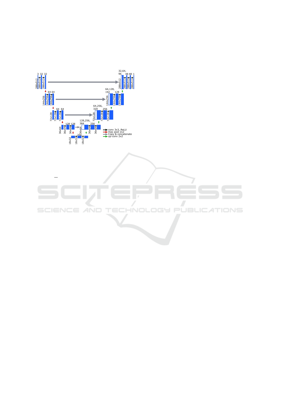
The architecture of neural network has been based

on the U-Net (Ronneberger et al., 2015) in which

we can distinguish a down-sampling (encoding) path

and an up-sampling (decoding) path, see Fig. 1. In

the down-sampling path there are ﬁve convolutional

blocks. Each block has two convolutional layers with

3 × 3 ﬁlters and stride equal to 1. Down-sampling is

realized by max pooling with stride 2 × 2 that is ap-

plied on the end of every blocks except the last one.

In the up-sampling path, each block begins with a de-

convolutional layer with 3 × 3 ﬁlter and 2 × 2 stride,

which doubles the dimension of feature maps in both

directions and decreases the number of feature maps

by two. In each up-sampling block, two convolutional

layers decrease the number of feature maps, which

arise as a result of concatenation of deconvolutional

feature maps and the feature maps from correspond-

ing block in the encoding path. Finally, a 1 ×1 convo-

lutional layer is used. The neural network was trained

on RGB images of size 288 × 512. In order to reduce

training time, prevent overﬁtting and increase perfor-

mance of the U-Net we added Batch Normalization

(BN) (Ioffe and Szegedy, 2015) after each Conv2D.

BN is a kind of supplemental layer that adaptively

normalizes the input values of the following layer,

mitigating the risk of overﬁtting. Since it improves

gradient ﬂow through the network, it reduces depen-

3D Model-based 6D Object Pose Tracking on RGB Images using Particle Filtering and Heuristic Optimization

691

dence on initialization and higher learning rates are

achieved. Data augmentation is useful for the reduc-

tion of overﬁtting and it has also been applied during

the network training.

Figure 1: Architecture of U-Net for object segmentation.

The pixel-wise cross-entropy has been used as the

loss function for object segmentation:

L = −

∑

i=1

log( ˆy

) + (1 − y

)log(1 − ˆy

)] (1)

where N stands for the number of training samples, y

is true value and ˆy denotes predicted value.

3 6D OBJECT POSE TRACKING

At the beginning of this Section we discuss 6D object

pose tracking using PSO. Then, in Subsection 3.1.2

we present the ﬁtness function. Afterwards, we

present 6D object pose tracking using particle ﬁlter-

ing. In Subsection 3.2.2 we outline observation and

motion models. Finally, in Subsection 3.3 we present

PF-PSO algorithm for 6D object pose tracking.

3.1 6D Object Pose Tracking using PSO

3.1.1 Particle Swarm Optimization

Particle swarm optimization (Kennedy and Eberhart,

1995; Sengupta et al., 2019) is an heuristic opti-

mization algorithm. It is derivative–free, stochastic

and population–based computational method, which

demonstrated a high optimization potential in un-

friendly non–convex, non–continuous spaces. The

swarm consists of a set of particles, and each swarm

member represents a potential solution of an opti-

mization task. The particles are placed in the search

space and move through such a space according to

rules, which take into account each particle’s personal

knowledge and the global knowledge of the swarm.

Every individual moves with its own velocity in the

multidimensional search space, determines its own

position and calculates its ﬁtness using an objective

function f (x). On the basis of the ﬁtness function the

particles determine the best locations and the global

best location.

The ordinary PSO algorithm begins by creating

particles at initial locations, and assigning them ini-

tial velocities (Kennedy and Eberhart, 1995). After-

wards, it determines the value of the objective func-

tion at each particle location, as well as determines

the best function value and the corresponding best lo-

cation. It determines new velocities, based on the cur-

rent velocity, the particles’s individual best locations,

and the best location of the entire swarm. In his work,

a topology with the global best has been selected due

to its faster convergence in comparison to neighbor-

hood best one.

At the beginning of optimization, each particle is

initialized with a random position and velocity. While

seeking the best ﬁtness, every individual i is attracted

towards a position, which is affected by the best po-

sition p

(i)

found so far by itself and the global best

position p

found by the whole swarm. In every iter-

ation k, each particle’s velocity is ﬁrst updated based

on the particle’s current velocity, the particle’s local

information and global information discovered by the

entire population. Then, each particle’s position is

updated using the velocity. In the ordinary PSO, the

position and velocity are calculated as follows:

(i)

k+1

= wv

(i)

+ c

(i)

− x

(i)

) + c

(i)

g,k

− x

(i)

)

(2)

(i)

k+1

= x

(i)

+ v

(i)

k+1

(3)

where w is the positive inertia weight, v

(i)

is the ve-

locity of particle i, r

(i)

and r

(i)

are uniquely generated

random numbers with the uniform distribution in the

interval [0.0, 1.0], c

, c

are positive constants, p

(i)

the best position that the particle i has found so far,

denotes the best position that was found by any

member of the swarm.

Equation (2), which updates the particle velocity

has three main components. The ﬁrst component that

is frequently referred to as inertia models the parti-

cle’s tendency to keep it moving in the same direction

it was moving previously. In fact it controls the ex-

ploration of the search space. The second component,

called cognitive, attracts the particle towards the best

position p

(i)

that was found formerly. The last com-

ponent is referred to as social and it pulls the particle

towards the best position p

found by any particle.

The ﬁtness value that corresponds to p

(i)

is called lo-

VISAPP 2020 - 15th International Conference on Computer Vision Theory and Applications

692

cal best p

(i)

best

, whereas the ﬁtness value corresponding

to p

is deﬁned as g

best

. We implemented an asyn-

chronous PSO, where in a given iteration, each par-

ticle updates and communicates its state to particles

after its move to a new position, see pseudo-code of

PSO algorithm. This means that the particles that will

be updated in the same iteration can exploit the new

best position immediately, instead of using the global

best calculated in the previous iteration.

1 function PSO(X, iter)

2 for k = 0 to iter − 1 do

3 for each particle x

(i)

∈ X do

4 f x = f (x

(i)

)

5 if f x < p

(i)

best

then

6 p

(i)

= x

(i)

7 if f x < g

best

then

8 p

= x

(i)

9 v

(i)

← update velocity using (2)

10 x

(i)

← update position using (3)

11 endfor

12 endfor

13 return p

The discussed algorithm is typically employed for

solving static optimization problems. The tracking of

the 6D object pose can be accomplished by dynamic

optimization and incorporating the temporal continu-

ity information into normal PSO. This means that

the 6D object pose can be estimated by a sequence

of static PSO-based optimizations, followed by re-

diversiﬁcation of the particles to generate a search

area containing the potential object poses that can

arise in the next frame. The re-diversiﬁcation of the

particle i can be obtained on the basis of normal dis-

tribution concentrated around the best particle loca-

tion p

in time t − 1, which can be expressed as:

(i)

← N (p

,Σ), where x

(i)

stands for particle’s lo-

cation in time t, Σ denotes the covariance matrix of

the Gaussian distribution, whose diagonal elements

are proportional to the expected movement.

3.1.2 Fitness Function

In recent years the PSO has been successfully applied

in several model-based applications, including object

detection (Ugolotti et al., 2013) and 3D pose reﬁne-

ment via rendering and texture-based matching (Zab-

ulis et al., 2014). In 3D model-based tracking of 6D

object pose the most computationally demanding op-

eration is computing the objective function. A sub-

stantial speed-up of computation of the ﬁtness func-

tion can be attained on modern GPU devices (Rymut

et al., 2013). In this work, more attention is paid to

reliable segmentation of the object of interest as well

as tracking accuracy of 6D object pose, and thus the

focus is on CPU implementation of ﬁtness function to

simplify design and evaluation of various algorithms.

In PSO-based approach every particle represents

a hypothesis about likely 6D pose of the object. The

ﬁtness score of the particle is calculated by project-

ing the 3D model and then matching the projected

model with the current image observations. Our ﬁt-

ness score depends on the ratio of overlap between

rasterized 3D model in the hypothesized pose and the

segmented object. The overlap ratio is the sum of

the overlap degree from the object shape to the ras-

terized model and the overlap degree from the raster-

ized model to the object shape. The larger the over-

lap ratio is, the larger is the ﬁtness value. Our ﬁt-

ness function includes also the normalized distance

between the model’s projected edges and the closest

edges in the image. The discussed factor is calculated

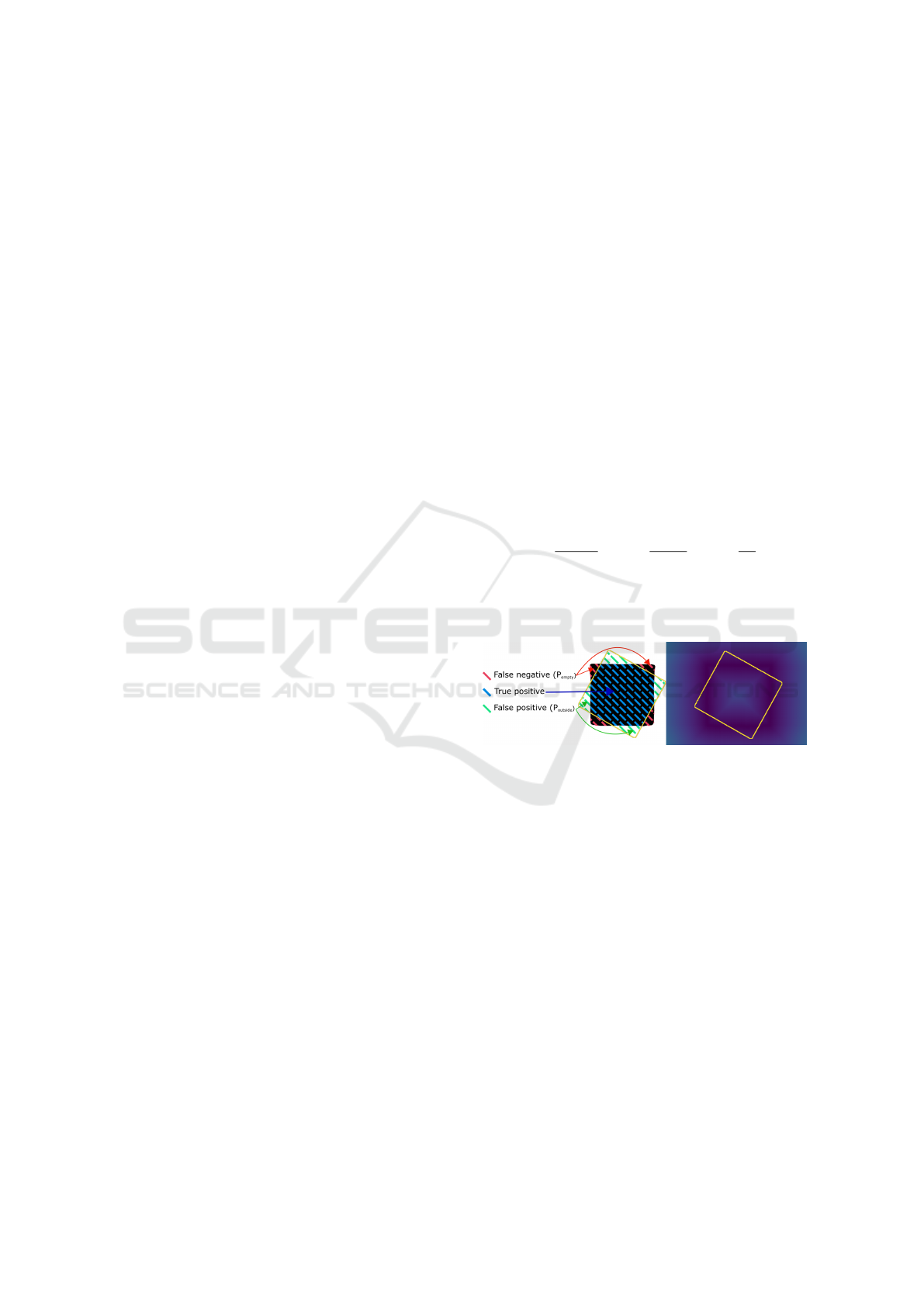
on the basis of the edge distance map, see Fig. 2.

The ﬁtness score is calculated as follows:



0.5 ∗

outside

model

+ 0.5 ∗

empty

seg



∗





(4)

where P

outside

stands for number of pixels projected

from model that are outside of segmented object on

image, see also Fig. 2 (left),

Figure 2: Fitness function.

model

denotes number of pixels in the projected

model, P

empty

is number of pixels of segmented object

on the image that are not covered by projected model,

seg

stands for number of pixels from segmented ob-

ject, K is sum of L2 distance transform values from

projected model’s edges to object edges on the image,

see Fig. 2 (right), P

denotes number of edge pixels in

the projected object outline, and w

= 0.4, w

= 0.6

are exponents that were determined experimentally.

3.2 6D Object Pose Tracking using PF

3.2.1 Particle Filtering

Particle ﬁlters permit estimating the state of partially

observable controllable Markov chains, i.e. dynami-

cal systems. For state estimation a probabilistic model

of the system and a probabilistic observation model

are needed. In this paper, the measurement at time t

3D Model-based 6D Object Pose Tracking on RGB Images using Particle Filtering and Heuristic Optimization

693

is denoted by z

, and x

denotes the state of the sys-

tem. Denoting by the superscript

all events leading

up to time t, the measurement can be expressed as:

= z

,.. .,z

. where the subscript

stands for an

event at time t. Particle ﬁlters, like other Bayes ﬁl-

ters, such as HMMs and Kalman ﬁlters, estimate the

posterior distribution p(x

) of the dynamical sys-

tem state conditioned on the data. This is done via the

following recursive formula:

p(x

) = η

p(z

)

p(x

t−1

)p(x

t−1

)dx

t−1

(5)

where η

is a normalization constant. To determine

the posterior three probability distributions, which are

referred as the probabilistic model of the dynamical

system are needed: (i) a measurement model p(z

)

describing the probability of measuring z

when the

system is in state x

, (ii) a motion model p(x

t−1

)

characterizing the probability of transiting from the

state x

t−1

to the state x

, (iii) an initial state distribu-

tion describing the initial system state.

A particle ﬁlter represents probability density

function (PDF) of nonlinear/non-Gaussian system by

a set of random samples. It is a common method to

cope with non-Gaussian noises. The posterior PDF

is approximated by a set of samples with associated

weights: X

= {x

[i]

}

i=1,...,m

. Such particle set approx-

imates the posterior p(x

). Initially, at time t = 0,

the particles x

[i]

are drawn from the initial state distri-

bution p(x

). Given X

t−1

, the particle set X

is then

calculated recursively in the following manner:

1 function PF(X

t−1

)

2 set X

= X

3 for j = 1 to m do

4 pick the j-th sample x

[ j]

t−1

∈ X

t−1

5 draw x

[ j]

∼ p(x

[ j]

t−1

)

6 set w

[ j]

= p(z

[ j]

)

7 add hx

[ j]

i to X

8 endfor

9 for i = 1 to m do

10 draw x

[i]

from X

with prob. ∝ to w

[i]

11 add x

[i]

to X

12 endfor

13 return X

In lines 2 through 10 a new set of particles is gener-

ated on the basis of the estimate X

t−1

of the previous

time step through incorporating the probabilistic mo-

tion model, the probabilistic observation model and

a resampling. Thus, the particle ﬁlter estimates recur-

sively the particle set X

on the basis of X

t−1

. For large

m the resulting weighted particle set is asymptotically

distributed according to the desired posterior.

3.2.2 Motion and Observation Models

The probabilistic observation model is as follows:

p(z

) = exp(− f

/σ

), where σ

is variance chosen

experimentally. Particles are propagated according to

a Gaussian distribution parameterized by σ

, which

was determined experimentally.

3.3 Proposed PF-PSO

The motivation is to improve the PSO by enabling

the algorithm dealing with multi-modal distributions.

At the beginning of each frame a PF is executed to

determine the posterior distribution. Then, samples

are clustered using k-means++ (Arthur and Vassilvit-

skii, 2007) algorithm, which applies a sequentially

random selection strategy according to a squared dis-

tance from the closest center already selected. Then,

a PSO with two sub-swarms consisting of samples as-

signed to the clusters is executed to ﬁnd the modes in

the probability distribution. The number of the itera-

tions in the PSO is set to three. Afterwards, ten best

particles are selected to form a sub-swarm, see lines

#5-6 in below pseudo-code. Twenty iterations are ex-

ecuted by such a particle sub-swarm to ﬁnd better par-

ticle positions. The best global position returned by

the discussed sub-swarm is used in visualization of

the best pose. Finally, an estimate of the probability

distribution is calculated by replacing the particle po-

sitions determined by the PF with corresponding par-

ticle positions, which were selected to represent the

modes in the probability distribution, see lines #5-6,

and particles reﬁned by the sub-swarm, see line #8.

The initial probability distribution is updated by ten

particles with better positions found by the PSO algo-

rithms and ten particles with better positions found by

the sub-swarm, see lines #9-11.

1 function select(n best,X)

2 X

sorted

= quicksort(X) using f ()

3 return X

sorted

[1.. .n best]

1 X

= PF(X

t−1

)

2 X

= k-means++(X

)

3 ∼,X

= PSO(X

,3)

4 ∼,X

= PSO(X

,3)

5 X

c1 best

= select(5,X

)

6 X

c2 best

= select(5,X

)

7 X

best

= X

c1 best

c2 best

8 g

best

= PSO(X

best

,20)

9 substitute 5 x ∈ X

with corresp. x ∈ X

c1 best

10 substitute 5 x ∈ X

with corresp. x ∈ X

c2 best

11 substitute 10 x ∈ X

with corresp. x ∈ X

best

12 return g

best

VISAPP 2020 - 15th International Conference on Computer Vision Theory and Applications

694

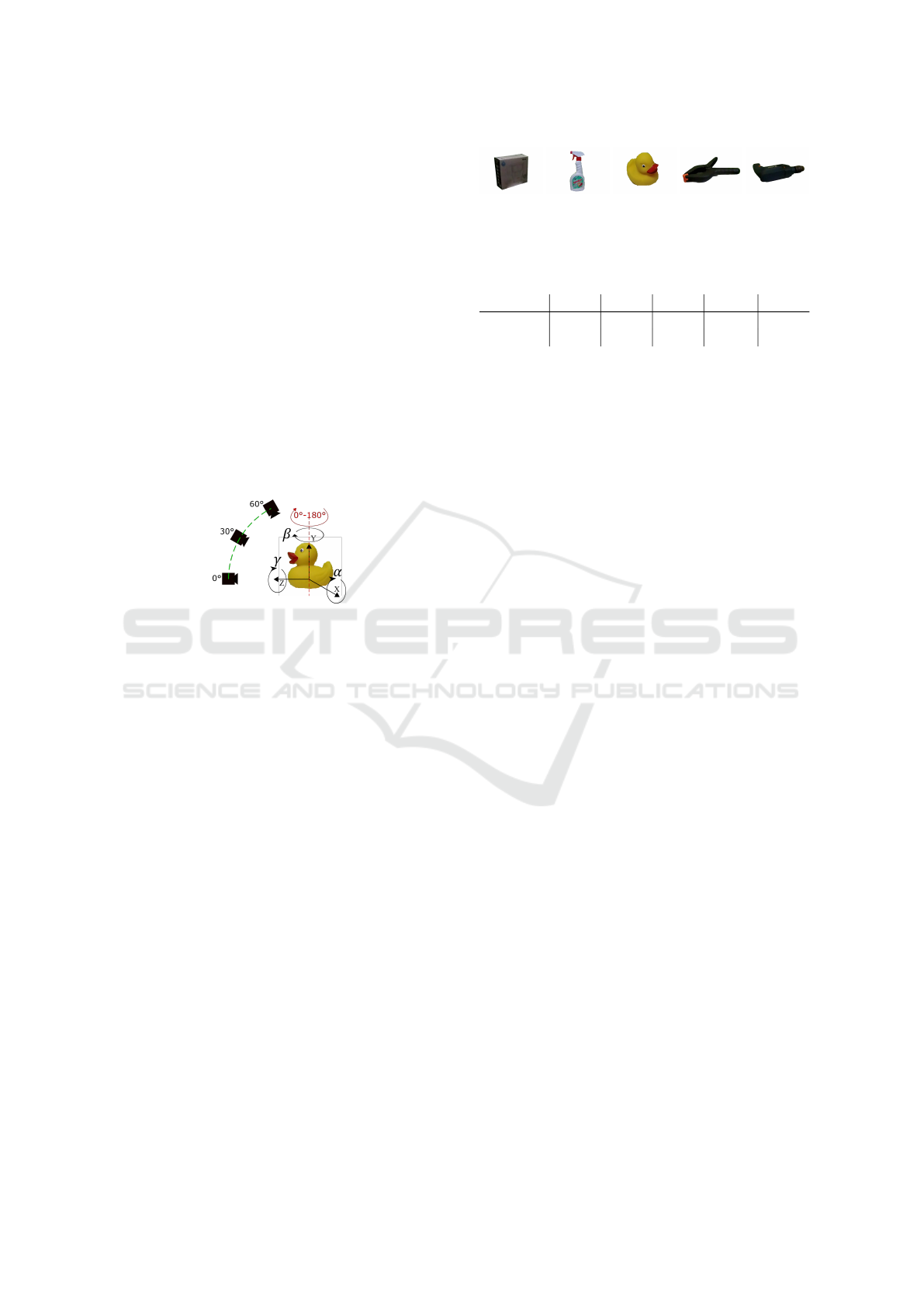
4 EXPERIMENTAL RESULTS

The experimental evaluation has been performed on

ﬁve objects: box, bottle, duck, clamp and drill. The

selected objects are almost entirely without any tex-

ture. 3D models of objects were created using the

Kinect 2.5D RGB-D camera (Izadi et al., 2011) and

SfM techniques. The OpenCV library (Bradski and

Kaehler, 2013) has been used to calibrate the RGB

camera. The ground truths of the object poses have

been obtained by a turnable device, on which each

object has been placed and then observed from three

different camera views, see Fig. 3. For each camera

view the objects were rotated in range 0

◦

... 180

◦

, and

nineteen images were recorded. During object rota-

tion, an image has been acquired every ten degrees

with information about corresponding rotation angle.

Each experiment has been repeated three times, the

error metrics were calculated and then averaged.

Figure 3: Experiments setup.

In order to learn the segmentation model the con-

sidered objects were observed by the camera from dif-

ferent views. For each object more than one hun-

dred manual delineation of objects were done and

then used to train neural networks for object segmen-

tation. The models trained in such a way were then

used to segment the objects from the background. Af-

terwards, a dataset consisting of RGB images with the

corresponding ground truth data has been stored for

the evaluation of algorithms for 6D object pose esti-

mation and tracking.

4.1 Object Segmentation

A single U-Net neural network discussed in subsec-

tion 2 has been trained to segment the considered ob-

ject using the set of manually segmented images. Ta-

ble 1 presents the Dice scores achieved on the test

subset of the dataset. The test subset contains thirty

images for each object. As we can observe in Tab. 1,

promising segmentation results were achieved for U-

Net trained separately for each of the considered ob-

jects. Having on regard a better usefulness of a sin-

gle U-Net for segmentation of all ﬁve objects, in the

following subsections we present the experimental re-

sults achieved on the basis of the common U-Net for

all ﬁve objects, see sample results on Fig 4.

Figure 4: Segmented objects.

Table 1: Dice scores on the test sub-dataset (ind. stands for

individual U-Net for each object, whereas common means

a common U-Net for all objects.

U-Net box bottle duck clamp drill

ind. 0.985 0.964 0.974 0.971 0.928

common 0.946 0.972 0.978 0.968 0.965

4.2 Experimental Evaluation

We conducted experiments consisting in tracking the

6D object pose in sequences of RGB images. The ob-

jects were observed from different views. The exper-

iments were performed on sequences of RGB images

of size 288 × 512 acquired in advance and stored in

mp4 ﬁles. For every camera view, the 6D pose of each

object has been tracked on nineteen images. The ob-

jects were rotated about the vertical axis with poses

changed about ten degrees. We evaluated the qual-

ity of 6-DoF object pose estimation using ADD score

(Hinterstoisser et al., 2013). The 6D object pose esti-

mate is considered valid if the ADD is smaller than

ten percent of object’s diameter. Table 2 presents

scores [%] achieved by trackers on box [ADD < 3.5

cm], bottle [ADD < 2.6 cm], duck [ADD < 1.5 cm],

clamp [ADD < 2.2 cm] and drill [ADD < 3.0 cm].

The PF-PSO simple is a simpliﬁed version of the PF-

PSO, where no k-means++ clustering has been exe-

cuted, i.e. single PSO executing three iterations has

been employed. As we can notice in Tab. 2, the PF-

PSO achieves superior results on all objects except

the duck. The poses of symmetrical objects were

estimated with satisfactory accuracies with rotations

about vertical symmetry axes in range 0

◦

... 180

◦

The discussed results were achieved on the basis of

one thousand calls of the objective function in single

frame. The number of the calls of the ﬁtness function

in PF-PSO has been identical to number of the calls

performed by the ordinary PF or the ordinary PSO. A

multinomial resampling has been used in the PF. The

state vector consists of 3D position and three Euler

angles describing rotation about axes, see Fig. 3.

Table 3 presents ADD scores [%] achieved by PF-

PSO in 6D object tracking in 0

◦

, 30

◦

and 60

◦

camera

views. As we can notice, the reason that the PF-PSO

achieves worse results for the duck are bigger errors

for 60

◦

camera view.

Figure 5 presents plots of angle tracking errors

over time, which were achieved by the algorithms for

the bottle and the drill. As we can observe, the parti-

3D Model-based 6D Object Pose Tracking on RGB Images using Particle Filtering and Heuristic Optimization

695

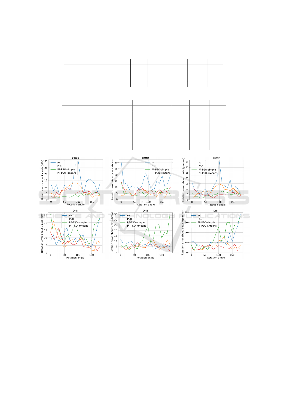
Table 2: Scores [%] achieved in 6D object tracking for box [ADD < 3.5 cm], bottle [ADD < 2.6 cm], duck [ADD < 1.5 cm],

clamp [ADD < 2.2 cm] and drill [ADD < 3.0 cm].

tracking score [%] box bottle duck clamp drill

PF, angle 0. . . 180

◦

0.345 0.222 0.246 0.281 0.450

PSO, angle 0. . . 180

◦

0.807 0.877 0.719 0.579 0.813

PF-PSO simple, ang. 0. . . 180

◦

0.889 0.912 0.351 0.520 0.614

PF-PSO, ang. 0. . . 180

◦

0.901 0.947 0.673 0.643 0.889

Table 3: Scores [%] achieved by PF-PSO in 6D object tracking.

tracking score [%] box bottle duck clamp drill

◦

camera view, angle 0. . . 90

◦

0.933 1.000 0.900 0.733 0.900

◦

camera view, angle 0. . . 180

◦

0.895 1.000 0.890 0.421 0.825

◦

camera view, angle 0. . . 90

◦

0.933 0.833 1.000 0.833 0.900

◦

camera view, angle 0. . . 180

◦

0.895 0.895 0.632 0.737 0.947

◦

camera view, angle 0. . . 90

◦

0.833 0.933 0.400 0.867 0.900

◦

camera view, angle 0. . . 180

◦

0.912 0.947 0.526 0.772 0.895

Average, angle 0. . . 90

◦

0.900 0.922 0.767 0.811 0.900

Average, angle 0. . . 180

◦

0.901 0.947 0.673 0.643 0.889

Figure 5: Pose errors over time for bottle and drill.

cle ﬁlter can continue tracking the object pose despite

currently larger errors in several consecutive frames,

see also errors about one hundred degrees for the bot-

tle. The errors achieved by the PF-PSO for speciﬁc

angle are smaller than 10

◦

, except the error in a few

frames for the drill, where in x axis, see Fig. 3, it is

slightly bigger than ten degrees.

In experiments with pose tracking algorithms we

noticed that the ordinary PSO can achieve promising

results. However, in tracking the 6D pose of more

complicated objects, the ordinary PSO can have dif-

ﬁculties with the tracking due to selecting in a given

frame a mode, which in next frames will not allow to

seek the optimal pose. On the other hand, the pro-

posed PF-PSO contains particles representing worse

mode in the given frame, which can be useful and can

give better results in forthcoming frames.

The complete system for 6D pose estimation and

tracking has been implemented in C/C++ and Python.

The system runs on an ordinary PC with a GPU card.

The images for training and evaluating the segmenta-

tion algorithm as well as extracted objects with cor-

responding ground-truth for evaluating the 6D ob-

ject pose estimation and tracking are freely available

for download at: http://home.agh.edu.pl/

∼

majcher/

src/visapp.

VISAPP 2020 - 15th International Conference on Computer Vision Theory and Applications

696

5 CONCLUSIONS

We have presented a 3D model based algorithm for

6D object pose tracking in sequence of RGB images.

The object has been segmented using U-Net neural

network. The 6D object pose estimation has been

performed by particle ﬁlter combined with particle

swarm optimization algorithm. Owing to clustering

particles representing the probability distribution in

the PF, the extracted modes were processed by PSO

to represent them by a few representative particles in

the reﬁned probability distribution. In future work we

are going to apply this algorithm for object manipula-

tion by Franka Emika. The initialization of the track-

ing will be done on the basis of pose regression neural

networks.

ACKNOWLEDGEMENTS

This work was supported by Polish National

Science Center (NCN) under a research grant

2017/27/B/ST6/01743.

REFERENCES

Arthur, D. and Vassilvitskii, S. (2007). K-means++: The

Advantages of Careful Seeding. In Proc. ACM-SIAM

Symp. on Discrete Algorithms, pages 1027–1035.

Brachmann, E., Krull, A., Michel, F., Gumhold, S., Shotton,

J., and Rother, C. (2014). Learning 6D object pose es-

timation using 3D object coordinates. In ECCV, pages

536–551. Springer.

Brachmann, E., Michel, F., Krull, A., Yang, M., Gumhold,

S., and Rother, C. (2016). Uncertainty-Driven 6D

Pose Estimation of Objects and Scenes from a Single

RGB Image. In IEEE Conf. on Computer Vision and

Pattern Recognition (CVPR), pages 3364–3372.

Bradski, G. and Kaehler, A. (2013). Learning OpenCV:

Computer Vision in C++ with the OpenCV Library.

O’Reilly Media, Inc., 2nd edition.

Deng, X., Mousavian, A., Xiang, Y., Xia, F., Bretl, T., and

Fox, D. (2019). PoseRBPF: A Rao-Blackwellized

Particle Filter for 6D Object Pose Tracking. In

Robotics: Science and Systems (RSS).

Doucet, A., Godsill, S., and Andrieu, C. (2000). On Se-

quential Monte Carlo Sampling Methods for Bayesian

Filtering. Statistics and Computing, 10(3):197–208.

Fischler, M. A. and Bolles, R. C. (1981). Random Sample

Consensus: A Paradigm for Model Fitting with Ap-

plications to Image Analysis and Automated Cartog-

raphy. Commun. ACM, 24(6):381–395.

Hinterstoisser, S., Holzer, S., Cagniart, C., Ilic, S., Kono-

lige, K., Navab, N., and Lepetit, V. (2011). Multi-

modal templates for real-time detection of texture-less

objects in heavily cluttered scenes. In Int. Conf. on

Computer Vision, pages 858–865.

Hinterstoisser, S., Lepetit, V., Ilic, S., Holzer, S., Bradski,

G., Konolige, K., and Navab, N. (2013). Model based

training, detection and pose estimation of texture-less

3D objects in heavily cluttered scenes. In Computer

Vision – ACCV 2012, pages 548–562. Springer.

Ioffe, S. and Szegedy, C. (2015). Batch normalization: Ac-

celerating deep network training by reducing internal

covariate shift. In ICML - vol. 37, pages 448–456.

Izadi, S., Kim, D., Hilliges, O., Molyneaux, D., Newcombe,

R., Kohli, P., Shotton, J., Hodges, S., Freeman, D.,

Davison, A., and Fitzgibbon, A. (2011). KinectFu-

sion: Real-time 3D Reconstruction and Interaction

Using a Moving Depth Camera. In Proc. ACM Symp.

on User Interface Soft. and Techn., pages 559–568.

Kennedy, J. and Eberhart, R. (1995). Particle Swarm Opti-

mization. In Proc. of IEEE Int. Conf. on Neural Net-

works, pages 1942–1948. IEEE Press, Piscataway, NJ.

Lepetit, V., Pilet, J., and Fua, P. (2004). Point matching as a

classiﬁcation problem for fast and robust object pose

estimation. In Proc. IEEE Conf. on Computer Vision

and Pattern Recognition, volume 2, pages II–II.

Marchand, E., Uchiyama, H., and Spindler, F. (2016).

Pose estimation for augmented reality: A hands-on

survey. IEEE Trans. on Vis. and Comp. Graphics,

22(12):2633–2651.

Rad, M. and Lepetit, V. (2017). BB8: A scalable, accurate,

robust to partial occlusion method for predicting the

3D poses of challenging objects without using depth.

In IEEE Int. Conf. on Comp. Vision, pages 3848–3856.

Ronneberger, O., Fischer, P., and Brox, T. (2015). U-

Net: Convolutional networks for biomedical image

segmentation. In MICCAI, pages 234–241. Springer.

Rymut, B., Kwolek, B., and Krzeszowski, T. (2013). GPU-

accelerated human motion tracking using particle ﬁl-

ter combined with PSO. In Adv. Concepts Intell. Vi-

sion Syst., LNCS, vol. 8192, pages 426–437. Springer.

Sengupta, S., Basak, S., and Peters, R. A. (2019). Parti-

cle Swarm Optimization: A survey of historical and

recent developments with hybridization perspectives.

Machine Learning and Knowl. Extr., 1(1):157–191.

Ugolotti, R., Nashed, Y. S. G., Mesejo, P., Ivekovi

v., Mussi, L., and Cagnoni, S. (2013). Particle

Swarm Optimization and Differential Evolution for

Model-based Object Detection. Appl. Soft Comput.,

13(6):3092–3105.

Vidal, J., Lin, C., and Mart

ı, R. (2018). 6d pose estima-

tion using an improved method based on point pair

features. In Int. Conf. on Control, Automation and

Robotics (ICCAR), pages 405–409.

Xiang, Y., Schmidt, T., Narayanan, V., and Fox, D. (2018).

PoseCNN: A Convolutional Neural Network for 6D

Object Pose Estimation in Cluttered Scenes. In

Robotics: Science and Systems XIV (RSS).

Zabulis, X., Lourakis, M. I., and Stefanou, S. S. (2014).

3D pose reﬁnement using rendering and texture-based

matching. In Computer Vision and Graphics, pages

672–679. Springer.

3D Model-based 6D Object Pose Tracking on RGB Images using Particle Filtering and Heuristic Optimization

697