Reliability Comparison of Routing Protocols for WSNs in Wide
Agriculture Scenarios by Means of η
L
Index
Marco Cagnetti
a
, Mariagrazia Leccisi
b
and Fabio Leccese
c
Dipartimento di Scienze, Università degli Studi “Roma Tre”, via della Vasca Navale n.84, Rome, Italy
Keywords: WSN, Routing Protocols, AODV, LEACH, PEGASIS, MPRR.
Abstract: A comparison between the most suitable routing protocols for WSNs applied in wide agriculture scenarios is
shown. The protocols, already present in literature, have been conceived to better manage the power budget
of the nodes and are particularly suitable to cover the energy issues that wide agriculture scenario can request.
This study aims to indicate which of the protocols eligible for this scenario is the most suitable. Comparative
simulation test will be shown.
1 INTRODUCTION
Although an ultimate definition has not provided yet
by the scientific community, the term Wireless
Sensor Network (WSN) is typically referred to a
network of spatially dispersed devices, even called
nodes, for the sensing of the around environment and
able to transfer the acquired data by means of wireless
communications (Shi & Perrig, 2004; Akyildiz et al.,
2002). Typically, the nodes should be characterized
by a low level of complexity, low dimensions and
their power consumption should be low (Leccese et
al., 2014; Leccese et al., 2017). Obviously, these
characteristics, so as the overall price of the nodes,
depend from the final use. Therefore, aims in which
high reliability and/or high power consumptions is
needed are generally more complex and expensive
than to nodes used in less challenging contexts (Iqbal
et al., 2017; Abruzzese et al., 2009; Ming et al. 2009;
D'Amato et al., 2012; Abruzzese et al., 2009; Pasquali
et al. 2016; Pasquali et al. 2017). From a
communication point of view, the nodes often respect
a hierarchical structure in which the lowest level is
composed by nodes that have not a direct access to
the outside. They can transmit data to neighbouring
nodes that route own data and received ones coming
from other nodes to an upper level node enabled to
transfer outside the data. This last node is called “sink
a
https://orcid.org/0000-0003-0198-5043
b
https://orcid.org/0000-0003-2775-637X
c
https://orcid.org/0000-0002-8152-2112
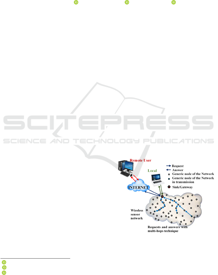
or gateway”. The ways to route the data and the way
to decide who will cover and how long depend by the
routing protocol implemented by the network.
Therefore, data locally acquired and gathered are
usually related to the sink by a routing based on
multiple hops that involve many nodes placed
between the farthest with respect to the sink. The sink,
making available the data to the outside, allows to
other clients to receive the information collected by
the local WSN. Fig. 1 shows an idea of a WSN
topology.
Figure 1: Typical architecture of a WSN.
Cagnetti, M., Leccisi, M. and Leccese, F.
Reliability Comparison of Routing Protocols for WSNs in Wide Agriculture Scenarios by Means of L Index.
DOI: 10.5220/0009365401690176
In Proceedings of the 9th International Conference on Sensor Networks (SENSORNETS 2020), pages 169-176
ISBN: 978-989-758-403-9; ISSN: 2184-4380
Copyright
c
2022 by SCITEPRESS – Science and Technology Publications, Lda. All rights reserved
169
The parameters on which working to design a
WSN are many and are linked to the scenario in which
it will be apply. In fact, as example, a WSN for a
smart city could not have electrical energy problems
because placed closed to the mains while, for an
application in open field far from the mains, the
procurement of power might be critical pushing the
designers to adopt all the possible solutions and
strategies to limit the power consumption.
Whithin of the design parameters, there are some
more evident, as the capacity of the batteries, and
other more complicated for which a deeper analysis
is necessary, as the routing protocols. In fact, the
energetic autonomy offered by a battery to a node is
directly proportional to its energy capacity. Instead,
for routing protocols that have different strategies to
route the data, it is more complicated to foresee their
impact on the power consumption of the nodes of the
WSNs. This is even more correct as some of them can
automatically change their setting during the time
(Al-Karaki & Kamal, 2004; Leccese et al., 2017).
In this paper, we are going to focus our attention
on the routing protocols trying to compare the
performance of existent protocols to find the more
suitable ones for an agricultural scenario in terms of
efficiency of the WSN. After a description of the
scenario in which we imagine to work, a description
of the routing protocols eligibile for this scenario will
be provided. At the end, a comparison between them
will be obtained by means of a suitable simulator.
2 OPERATIVE SCENARIO
The parameters involved in the definition of a WSN
are many, therefore, its designing is strongly
dependent by the scenario in which it is going to work
(Lamonaca et al., 2017; Gallucci et al., 2017; Morello
et al., 2010; D’Alvia et al., 2017; Islam et al., 2012;
Shen et al., 2001; Vicentini et al., 2014; Pecora et al.,
2019; Polese et al., 2019). For this reason, before any
consideration on the WSN, it is necessary to descript
the operative scenario. In our case, we considered a
wide agricultural site (WAS). We define a WAS as a
land of at least one hectare, in which there some kind
of crop. In order to simplify the geometry, but taking
nothing away from the generality of possible cases,
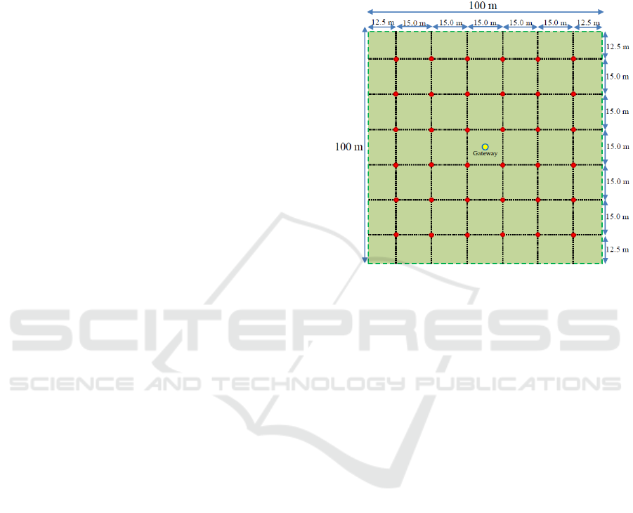
we imagine the soil flat and squared. Within of the
land, we decide to place a cert number of sensors that
depends by the needs. Fig. 2 gives an idea of the
placing of the sensors. The nodes (red circles) are
placed in the centres of an ideal grid made of internal
squares with a side of 15 m, therefore we could have
36 nodes for hectare, but this number is absolutely
aleatory and is fixed only to define a possible
operative scenario necessary for the further analysis.
Imaging that the land is far from farm, the nodes have
not the possibility to receive electrical energy from
the mains and have to be supplied by local sources as
batteries.
Figure 2: Possible operative scenario in which 36 nodes are
placed in a hectare of an agricultural land.
The use of other local electrical energy sources as
renewable ones, e.g. photovoltaic panels, is not
considered since the idea is to make as efficient as
possible the WSN. This leads a deep analysis of the
routing protocols because in order to increase as
much as possible the efficiency, the power
consumption of the WSN must be as low as possible.
Between the nodes placed in the land, we decided to
put the gateway in the centre of the WSN.
3 ROUTING PROTOCOLS
After the definition of a possible operative scenario,
which revealed the problem of power consumption
and so the need to make the network as efficient as
possible, a description of the routing protocols that in
literature are pointed out as the most suitable for this
kind of scenario is necessary. Between the routing
protocols present in literature four of them seem
suitable for our scenario: Ad hoc On Demand
Distance Vector routing protocol or AODV (Maurya
et al., 2012), Low-Energy Adaptive Clustering
Hierarchy or LEACH (Shekar, 2012), Power-
Efficient GAthering in Sensor Information Systems
or PEGASIS (Lindsey, 2013) and Multipath Ring
Routing or MPRR (Pandya & Mehta, 2012).
WSN4PA 2020 - Special Session on Wireless Sensor Networks for Precise Agriculture
170

3.1 AODV
The Ad-hoc On-Demand Distance Vector (AODV) is
a reactive protocol principally conceived for ad hoc
mobile networks and is able to set both unicast and
multicast routing. It builds routes between nodes only
as desired by source nodes (in this sense, it is an on
demand algorithm) maintaining they active until is
requested by the source nodes. All the routing
information are uploaded in a routing table driven,
and so updated, by the demand reducing the typical
problem of the proactive routing protocols which try
to up to date all the time the routing tables engaging
many computational resources.
For destination, AODV uses sequence numbers
that avoid routing loops so preventing problems such
as the "counting to infinity" more typical for more
classical distance vector protocols.
Other advantages are the quick adaptation to
dynamic link evolutions, a low overhead of
processing and memory, it has the ability to find
unicast routes to destinations within the ad hoc
network, self-starting and scales to large numbers of
mobile nodes.
Unfortunately, this protocol presents problems in
case of managing of network congestion where an
overloading of nodes is typical. This makes slower
the transmission speed of the network but, even more
important from our point of view, the nodes should be
energetically weaker.
3.2 LEACH
Low Energy Adaptive Clustering Hierarchy
(LEACH) is conceived for hierarchical clustering
WSNs. A cluster is a set of nodes that, in order to
make similar the power consumption, randomly, after
a fixed time, elects a cluster-head (CH) rotating this
role between the nodes within of the cluster. The CHs
collects data coming from the nodes aggregate them
and compress the total amount of information that
will be send to the base station (BS). In MAC layer, a
TDMA/CDMA technique is implemented to reduce
the possible collisions inside the cluster or between
different clusters. The collection of data is centralized
and can be set both periodically or asynchronously
making it suitable to constant monitoring activities.
The set-up of the WSN is performed in two
successive steps called setup phase and steady state.
During the setup, there is the organization of the
clusters which elect the own CHs while, in the second
phase, the data transfer inside the cluster and to the
BS is done. The procedure foresees that during the
setup phase, a small number of nodes elect
themselves as CHs notifying their own role to the
other nodes using a broadcast message. The other
nodes, alerted by this message, on the base of the
signal strength, decide on which cluster they want to
belong informing the appropriate CHs that they are a
member of that cluster. Once established the cluster,
a TDMA schedule is established by the CH node,
which assigns a time slot to each node for the
transmission. This schedule is sent to the other nodes
of the cluster through a broadcast message. During
the steady state phase, the data are transmitted. After
an aforethought time, a new setup phase is launched.
The principal advantage of the LEACH protocol
is the high lifetime of the network. On the contrary, it
assumes that all nodes have enough power to transmit
to reach the BS and that each node has been designed
to work with different MAC protocols. Therefore, if
the network is not properly designed, its application
for networks deployed in large regions could be
critical. Another disadvantage is the fact that it is not
ensured that the CHs are uniformly distributed in the
network having the possibility that the CHs can be
concentrated only in a part of the network. This
implies that some nodes may not be close to CHs.
Another disadvantage is that the dynamic clustering
leads further overhead caused by head changes,
advertisements etc., which drains the available
energy. Moreover, the protocol supposes that, at the
beginning, all nodes have the same quantity of energy
in each round, wrongly assuming that each CH
consumes a similar quantity of energy.
3.3 PEGASIS
Power-Efficient GAthering in Sensor Information
Systems can be considered as an optimization of the
LEACH algorithm. It does not group nodes in clusters
but forms chains of sensor nodes. With this
architecture, each node talks only with the closest
neighbors receiving and transmitting data only from
the previous ring and with successive ring of the
chain. In this way, the nodes can adjust the power of
their transmissions. Even in this case, the single node
performs the aggregation of data coming from the
previous with own and forwarding the new set to the
next node of the chain up to the BS. Each round,
foresees that one node of the chain is elected to
communicate with the BS and the chain is built
according to a greedy algorithm. The final packet that
will be sent out of the WSN is made with the data
collected from all nodes so realizing a “data fusion.”
This texture has the great advantage to reduce the
overall amount of the data transmitted to the BS
because reduces the number of ancillary data that
Reliability Comparison of Routing Protocols for WSNs in Wide Agriculture Scenarios by Means of L Index
171

forms, together with the measured information, the
data packet coming from a single sensor.
With respect to the LEACH, the main
advantageous of the Pegasis is the lower transmission
distance between the nodes, moreover, since the
nodes are selected for only the time of the
transmission round, the power dissipation during the
time is balanced between the nodes. On the contrary,
PEGASIS presents many disadvantages:
requests that the CHs have to be located near the
BS;
since the energy of the CH at the beginning is
unknown, there is the risk that the nodes could
discharge during a transmission losing all the data
coming from the whole WSN;
the presence of an only CH could be a bottleneck
for the network causing delays;
the lack of redundancy increase the risk of lost;
if the packets have a low number of bits, the
energy efficiency is low.
3.4 MPRR
In order to make data collection robust against
communication failures, multipath routing
architectures allow setting up multiple propagation
paths between each sensor node and the base station.
In this way, data collected by a node are successfully
sent to the base station as long as any one of its
propagation paths is failure-free (Huang et al., 2013).
In MPRR, nodes do not have a specific parent and
the construction phase organizes the network into
levels, even called rings, according to hop distance
from the sink node to a sensor node. This means that,
at the end of the build phase, each node will have a
number that indicates how many hops is far from the
sink node and this number corresponds to the level or
ring of belonging.
At the beginning of the construction phase, the BS
sends a broadcast setup packet indicating the ring
number 0. The nodes that receive this topology setup
packet will increment it 1 (nodes belonging to ring 1)
and rebroadcast it. This process continues until all
nodes will have a ring number. After topology setup
phase is completed, when a node needs to send data
to the gateway, the node sends a broadcasts message
endowed of its ring number. Any node having a
smaller ring number will receive that packet and
rebroadcasts it. The process continues until the packet
reaches to sink. In this sense, MPRR is a proactive
routing protocol in which the network initialization is
performed prior to the data dissemination, all nodes
are distributed randomly in the field under analysis,
the base station is responsible for gathering data from
the whole network, moreover, route discovery is also
not required before data transmission.
Because of its own architecture, MPRR is natively
reliable in the transmission data; in fact, the
possibility to set more paths to reach the sink ensures
that the data sent by the generic sensor node has more
possibility to reach the gateway respect to a less
complex topology. On the contrary, the major
disadvantage is the overall overhead of the WSN that
drains inefficiently energy from the nodes.
4 CASTALIA SIMULATOR
In order to study the most suitable routing protocol
for the described agricultural scenario, we used a
WSN simulator able to implement low-power
embedded devices: its name is Castalia. We chose this
simulator since it is “open source.” This allows
studying the algorithm following step by step what
happens during the simulations verifying the
compliance of the software with the theory and allows
introducing check points to avoid problems as infinite
loops, etc. At the same time, it allows modifying
already defined algorithms, and, even more
important, allows implementing, developing and
validating new algorithms (Boulis, 2019). Anyway,
in order to find the best protocols, we decided to not
change the already algorithms testing the original
version of the protocols implemented in the
simulator.
5 TEST AND RESULTS
A comparison between different routing protocols
can be scientifically insignificant because each
protocol has been conceived to exalt some
characteristics with respect to the others. For instance,
AODV has been conceived for mobile networks and
surely will better fit to the exigencies of those nets
instead of static architectures. This leads that the test
are typically focused on a single aspect (resilience,
energy consumption, transmission speed, etc.)
analysing how and how much a specific protocol is
better than the other for that specific aspect. Although
this approach is overall reasonable because there is
not a perfect WSN for all possible scenario, in order
to try a more suitable and objective index for our test,
we used a performance index that takes into account
both the energy aspects and the reliability of data
transmission.
WSN4PA 2020 - Special Session on Wireless Sensor Networks for Precise Agriculture
172
5.1 Performance Index
The index, called η
L
, is defined as the number of
packets received by the sink after a fixed time divided
for the difference between the initial nodes and those
that during the activity are switched off.
(1)
where:
η
L
: performance index
N
p: number of packet received by the sink after a
fixed time.
S: number of initial nodes (they are initially active.)
D: number of dead nodes after a fixed time.
For dead nodes, we mean even those unable to
communicate with the gateway. The index gives an
indication of how much efficient the network is in the
delivery of the information considering both the
number of packets that are running in the network and
that arrive to the sink and the number of nodes that
fail over the time. This fail could be linked to the
energy lack caused by the stress that some nodes
could suffer due to the strategy adopted by the routing
protocols. The index is built to have values lower,
higher or equal the unit value that represents the ideal
performance of the network in which the number of
the received packets is equal to the number of alive
nodes. This condition is certainly achieved by
protocols that do not provide redundancy in the
transmission of data and at a time (necessarily initial)
in which all the nodes are "alive". Numbers different
by the unit mean inefficiency: higher values indicate
that there is plenty of packets; lower values indicate
fewer packets than the number of live nodes.
5.2 Test, Results and Discussion
To perform the test, it has been assumed that each
sensor node is powered by on board battery (Caciotta
et al., 2013; Leccese, 2007). Additionally the battery
cannot be replaced or recharged, therefore the battery
discharge leads the failure of the node and determines
the lifetime of the WSNs. Considering the supposed
scenario of Fig. 2, it is assumed that one of the node
will perform the role of gateway. Moreover, the
quantity of data transmitted toward the gateway from
each node is equal for each routing protocol. It is clear
that in each epoch, depending on the specific
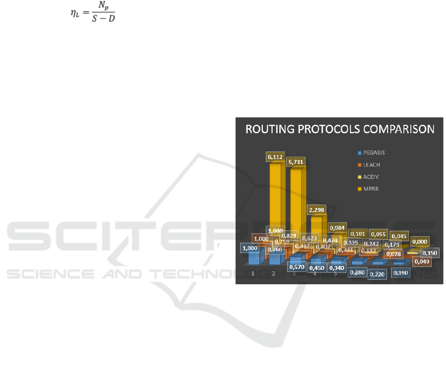
protocol, a certain percentage of nodes fail. Fig. 3
shows the average of 100 simulations obtained by
Castalia for a network composed of 100 nodes.
Consequently, the dimension of the hypothetical area
analyzed with the simulation is bigger than one
hectare. The numbers on the abscissas of the graphs
(from 1 to 8) indicate the evolution of the time
expressed in epochs (in real cases an epoch could be
equal to 2 months).
As it is possible to see, in the first epoch, the first
three protocols are similar showing optimal results,
while the MPRR shows high inefficiency cause the
redundancy of the packets that are running in the
network. High inefficiency does not mean that the
packets do not arrive to the sink, but simply that the
number of packets is redundant and so a high-energy
consumption without a real necessity happens.
After the first epoch, the first three protocols lose
efficiency, while the MPRR recovers efficiency even
if the improvement is strongly limited for the second
and for the third epoch.
Figure 3: Service performance index with respect to the
protocol: number of packets arrived at the SINK divided by
the difference between the number of initial nodes and
those switched off. Simulation obtained with CASTALIA
for a network of 100 nodes. The values are the average of
100 simulations; each simulation needs about 40 minutes to
be performed for a total simulation time of about 100 hours.
Between the first three protocols, the networks
managed by LEACH is surely weaker if compared
with PEGASIS and AODV. This can be explained
with the distribution of the dead nodes that is linked
to the protocol: in fact, in the LEACH, the CHs are
more stressed with respect to the other nodes even if
they are normally a limited number. Moreover, the
probability to select the CHs is higher for the nodes
nearer to the sink. The better performance of the
PEGASIS with respect the LEACH is due to the fact
that it is an improved version of this last, while the
good behavior of the AODV could be due to the
particular scenario. The behavior of the MPRR needs
some explanations. Considering how its routing
protocol works, it is highly inefficient at the
Reliability Comparison of Routing Protocols for WSNs in Wide Agriculture Scenarios by Means of L Index
173
beginning even if, in the first epochs, it ensures the
highest reliability of the network because all the
packets find a route to arrive to the sink. Always
considering its way to work, the nodes in the lower
levels are energetically more stressed than those
belonging to the upper levels and far from the
gateway. This leads an early death of the nodes
belonging to lower levels with respect to the other
routing protocols and this prevents to the nodes of the
higher levels to communicate with the gateway.
Therefore, even if many nodes of the higher rings are
still alive, they cannot communicate with the gateway
and so are considered died. This justifies its behavior
highly reliable at the beginning but that early
becomes unsuitable. In fact, after the fourth epochs,
the number of dead nodes belonging to the lower
rings is such as to prevent an acceptable transfer of
information. The simulations were performed on an
ASUS Notebook, with an Intel Core Pentium i7-
3630QM CPU @ 2.40 GHz and memory RAM of 8
GB. Each simulation took 40 minutes.
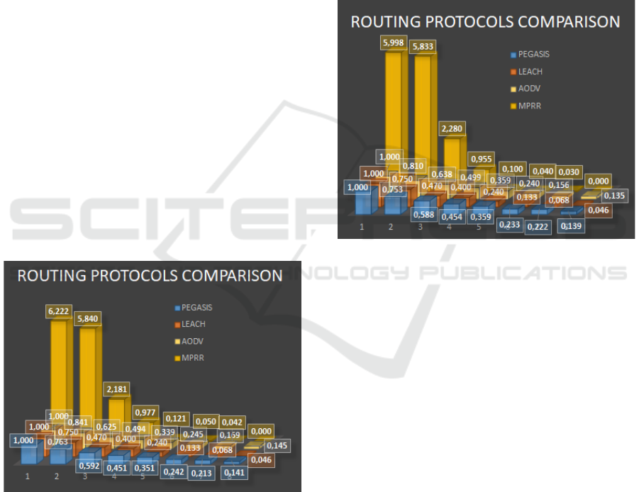
In order to validate our test we repeated the it with
a bigger number of nodes. The second test used 200
nodes and each simulation needs about 100 minutes
to be performed and a total simulation time of about
6 days. 300 nodes composed the third network and the
simulation needs about 360 minutes. In this case, we
performed only 50 simulations for a time of about
12,5 days. The results are shown in figures 4 and 5.
Figure 4: Service performance index with respect to the
protocol. Simulation obtained with CASTALIA for a
network of 200 nodes. The values are the average of 100
simulations; each simulation needs about 100 minutes to be
performed for a total simulation time of about 6 days.
As it is possible to see, even in these cases, the
graphs show that we have similar answers for similar
protocols (LEACH and PEGASIS) with PEGASIS
better than LEACH, while different architectures
(MPRR) suggest high reliability of the transmission
only for a short time. Anyway, even if the differences
between PEGASIS and AODV are not high, the
simulations identify in the AODV routing protocol a
good competitor for PEGASIS resulting both the
more suitable routing protocols for this scenario. This
leads that, if you have the possibility to change the
batteries of the nodes of if you have the possibility to
provide a safe and continuous energy source for the
nodes as the photovoltaic one, the better routing
protocols is surely the MPRR. If these possibilities
are not sure, a PEGASIS or an AODV could be the
better strategies for the WSN in this kind of scenario.
Figure 5: Service performance index with respect to the
protocol. Simulation obtained with CASTALIA for a
network of 300 nodes. The values are the average of 50
simulations; each simulation needs about 360 minutes to be
performed for a total simulation time of about 12.5 days.
6 CONCLUSIONS
In order to find a routing algorithm that can better fit
the exigencies of a wide agricultural scenario, a
comparison between the most suitable protocols
present in literature has been done by the use of a
particular performance index that points out how
many the network is reliable during the time. The
simulations have been realized with a scenario that
foresees an equally space spaced nodes in a flat land
with the gateway placed in the centre of the WSN,
with the nodes that start with the same amount of
energy and that send the same quantity of
information. This last choice is linked to the idea of
realizing the objective of the document without
possible facilitations. The simulations find that the
MPRR, although highly inefficient under the
energetic profile, ensures the deliverable of the
WSN4PA 2020 - Special Session on Wireless Sensor Networks for Precise Agriculture
174

information during the first epochs showing itself as
the most reliable but only for a limited time.
PEGASIS, being an improvement version of the
LEACH, shows a performance better of this last,
while, paradoxically, the simulations identify in the
AODV protocol, conceived for mobile networks, a
valid competitor of the PEGASIS. This result can be
due both to the particular scenario and to the energy
requests of the other routing protocols.
REFERENCES
Shi, E., & Perrig, A. (2004). Designing Secure Sensor
Networks. IEEE Wireless Communications, 11 (6), 38-
43. DOI:10.1109/MWC.2004.1368895
Akyildiz, I. F., Su, W., Sankarasubramaniam, Y. & Cayirci,
E. (2002). Wireless sensor networks: a survey.
Computer Networks, 38 (4), 393-422.
DOI:10.1016/S1389-1286(01)00302-4.
Leccese, F., Cagnetti, M., Ferrone, A., Pecora, A. & Maiolo
L. (2014). An infrared sensor Tx/Rx electronic card for
aerospace applications. Proceedings of the IEEE
International Workshop on Metrology for Aerospace,
6865948, 353-357.
DOI:10.1109/MetroAeroSpace.2014.6865948.
Leccese, F., Cagnetti, M., Sciuto, S., Scorza, A., Torokhtii,
K., Silva, E. (2017). Analysis, design, realization and
test of a sensor network for aerospace applications.
Proceedings of IEEE International Instrumentation and
Measurement Technology Conference (I2MTC), 1-6.
DOI:10.1109/I2MTC.2017.7969946.
Iqbal, Z., Kim, K. & Lee H. N. (2017). A Cooperative
Wireless Sensor Network for Indoor Industrial
Monitoring. IEEE Transactions on Industrial
Informatics, 13(2), 482-491, April 2017.
DOI:10.1109/TII.2016.2613504.
Abruzzese, D. Angelaccio, M. Giuliano, R. Miccoli, L. &
Vari, A. (2009). Monitoring and vibration risk
assessment in cultural heritage via Wireless Sensors
Network. Proceedings of 2nd Conference on Human
System Interactions, 568-573.
DOI:10.1109/HSI.2009.5091040.
Ming, X., Yabo, D., Dongming, L., Ping, X. & Gang, L.
(2008). A Wireless Sensor System for Long-Term
Microclimate Monitoring in Wildland Cultural
Heritage Sites. Proceedings of IEEE International
Symposium on Parallel and Distributed Processing
with Applications, pp. 207-214.
DOI:10.1109/ISPA.2008.75.
D'Amato, F., Gamba, P. & Goldoni, E. (2012). Monitoring
heritage buildings and artworks with Wireless Sensor
Networks, Proceedings of IEEE Workshop on
Environmental Energy and Structural Monitoring
Systems (EESMS), 1-6.
DOI:10.1109/EESMS.2012.6348392.
Abruzzese, D., Angelaccio, M., Buttarazzi, B., Giuliano,
R., Miccoli, L. & Vari, A. (2009). Long life monitoring
of historical monuments via Wireless Sensors Network.
Proceedings of 6th International Symposium on
Wireless Communication Systems, 570-574. doi:
10.1109/ISWCS.2009.5285215.
Pasquali, V., Gualtieri, R., D’Alessandro, G., Granberg, M.,
Hazlerigg, D., Cagnetti, M. & Leccese, F. (2016).
Monitoring and analyzing of circadian and ultradian
locomotor activity based on Raspberry-Pi. Electronics
(Switzerland), 5 (3), art. no. 58, .
DOI:10.3390/electronics5030058.
Pasquali, V., D'Alessandro, G., Gualtieri, R. & Leccese, F.
(2017). A new data logger based on Raspberry-Pi for
Arctic Notostraca locomotion investigations.
Measurement: Journal of the International
Measurement Confederation, 110, 249-256.
DOI:10.1016/j.measurement.2017.07.004.
Al-Karaki, J. N. & Kamal, A. E. (2004). Routing techniques
in wireless sensor networks: a survey. IEEE Wireless
Communications, 11 (6), 6-28.
DOI:10.1109/MWC.2004.1368893.
Leccese, F., Cagnetti, M., Tuti, S., Gabriele, P., De
Francesco, E., Ðurovi
ć-Pejčev, R. & Pecora, A. (2017).
Modified LEACH for Necropolis Scenario.
Proceedings of the IMEKO International Conference
on Metrology for Archaeology and Cultural Heritage,
23-25 October, 2017, Lecce, Italy.
Lamonaca, F., Sciammarella, P. F., Scuro, C., Carni, D. L.
& Olivito, R.S. (2018). Internet of Things for Structural
Health Monitoring. Proceeding of the Workshop on
Metrology for Industry 4.0 and IoT, MetroInd 4.0 and
IoT 2018, 95-100.
DOI:10.1109/METROI4.2018.8439038.
Gallucci, L., Menna, C., Angrisani, L., Asprone, D., Lo
Moriello, R.S., Bonavolontá, F. & Fabbrocino, F.
(2017). An embedded wireless sensor network with
wireless power transmission capability for the
structural health monitoring of reinforced concrete
structures. Sensors (Switzerland), 17 (11), 2566, .
DOI:10.3390/s17112566.
Morello, R., De Capua, C. & Meduri, A. (2010). Remote
monitoring of building structural integrity by a smart
wireless sensor network. Proceeding of the IEEE
International Instrumentation and Measurement
Technology Conference, I2MTC 2010, 1150-1154.
DOI:10.1109/IMTC.2010.5488136.
D’Alvia, L., Palermo, E., Rossi, S. & Del Prete, Z. (2017)
Validation of a low-cost wireless sensors node for
museum environmental monitoring. ACTA IMEKO, 6
(3), 45. DOI:
http://dx.doi.org/10.21014/acta_imeko.v6i3.454.
Islam, K., Shen, W. & Wang X. (2012). Wireless Sensor
Network Reliability and Security in Factory
Automation: A Survey. IEEE Transactions on Systems,
Man, and Cybernetics, Part C (Applications and
Reviews), 42 (6), 1243-1256.
DOI:10.1109/TSMCC.2012.2205680.
Shen, C. C., Srisathapornphat, C. & Jaikaeo C. (2001).
Sensor information networking architecture and
applications. IEEE Personal Communications, 8 (4),
52-59. DOI:10.1109/98.944004.
Reliability Comparison of Routing Protocols for WSNs in Wide Agriculture Scenarios by Means of L Index
175

Vicentini, F., Ruggeri, M., Dariz, L., Pecora, A., Maiolo,
L., Polese, D., Pazzini, L., Molinari Tosatti, L. (2014).
Wireless sensor networks and safe protocols for user
tracking in human-robot cooperative workspaces, in
Proceedings of the IEEE 23
rd
International Symposium
on Industrial Electronics (ISIE’14), June 2014, pp.
1274-1279.
Pecora, A., Maiolo, L., Minotti, A., Ruggeri, M., Dariz, L.,
Giussani, M., Iannacci, N., Roveda, L., Pedrocchi, N. &
Vicentini, F. (2019). Systemic approach for the
definition of a safer human-robot interaction, Factories
of the Future, Ed Springer Cham pp. 173-196
Davide Polese, Luca Maiolo, Luca Pazzini, Guglielmo
Fortunato, Alessio Mattoccia, Pier Gianni Medaglia,
Wireless sensor networks and flexible electronics as
innovative solution for smart greenhouse monitoring in
long-term space missions, Proceedings of the 2019
IEEE 5th International Workshop on Metrology for
Aerospace, pp. 223-226
Maurya, P. K., G. Sharma, V. Sahu, A. Roberts & M.
Srivastava. (2012). An Overview of AODV Routing
Protocol. International Journal of Modern Engineering
Research (IJMER), 2 (3), 728-732. Retrieved from:
www.ijmer.com/papers/vol2_issue3/AC23728732.pdf.
Shekar, R. (2012). LEACH and PEGASIS Protocol.
Retrieved from Mangalore University:
https://www.slideshare.net/ReenaShekar/leach-
pegasis.
Lindsey, S. & Raghavendra, C. S. (2013) PEGASIS:
Power-Efficient Gathering in Sensor Information
Systems. Computer Systems Research Department The
Aerospace Corporation P.O. Box 92957 Los Angeles,
CA 90009-2957. Retrieved from
http://ceng.usc.edu/~raghu/pegasisrev.pdf.
Pandya, A. & Mehta, M. (2012). Performance Evaluation
of Multipath Ring Routing Protocol for wireless Sensor
Network. Proceedings of First International
Conference on Advances in Computer, Electronics and
Electrical, 410 – 414. DOI : 10.15224/978-981-07-
1847-3-924.
Huang, G. M., Tao, W. J., Liu, P. S. & Liu, S. Y. (2013).
Multipath Ring Routing in Wireless Sensor Networks.
Applied Mechanics and Materials, 347–350, 701–705.
https://doi.org/10.4028/www.scientific.net/amm.347-
350.701.
Boulis, A. (2019). Castalia user’s manual. NICTA.
Retrieved from:
https://github.com/boulis/Castalia/blob/master/Casta
lia%20-%20User%20Manual.docx.
Caciotta, M., Leccese, F., Giarnetti, S. & Di Pasquale, S.
(2013). Geographical monitoring of electrical energy
quality determination: The problems of the sensors.
Proceedings of the International Conference on
Sensing Technology, ICST, art. no. 6727776, pp. 879-
883. DOI: 10.1109/ICSensT.2013.6727776.
Leccese, F. (2007). Rome: A first example of perceived
power quality of electrical energy. Proceedings of the
IASTED International Conference on Energy and
Power Systems, pp. 169-176.
WSN4PA 2020 - Special Session on Wireless Sensor Networks for Precise Agriculture
176
