
Classification of Students’ Conceptual Understanding in STEM
Education using Their Visual Attention Distributions: A Comparison of
Three Machine-Learning Approaches
Stefan K
¨
uchemann, Pascal Klein, Sebastian Becker, Niharika Kumari and Jochen Kuhn
Physics Department - Physics Education Research Group, TU Kaiserslautern,
Erwin-Schr
¨
odinger-Strasse 46, 67663 Kaiserslautern, Germany
Keywords:
Eye-tracking, Machine Learning, Deep Learning, Performance Prediction, Total Visit Duration, Problem-
solving, Line-graphs, Adaptive Learning Systems.
Abstract:
Line-Graphs play a central role in STEM education, for instance, for the instruction of mathematical con-
cepts or for analyzing measurement data. Consequently, they have been studied intensively in the past years.
However, despite this wide and frequent use, little is known about students’ visual strategy when solving line-
graph problems. In this work, we study two example line-graph problems addressing the slope and the area
concept, and apply three supervised machine-learning approaches to classify the students performance using
visual attention distributions measured via remote eye tracking. The results show the dominance of a large-
margin classifier at small training data sets above random decision forests and a feed-forward artificial neural
network. However, we observe a sensitivity of the large-margin classifier towards the discriminatory power
of used features which provides a guide for a selection of machine learning algorithms for the optimization of
adaptive learning environments.
1 INTRODUCTION
In times of increasing heterogeneity between learn-
ers, it becomes increasingly important to respond to
the needs of individuals and to support learners indi-
vidual learning process. One possibility is to person-
alize learning environments via adaptive systems that
are able to classify the learner’s behavior during the
learning or problem-solving process and potentially
include the knowledge of individual answers to pre-
vious questions which can produce a sharper picture
of learner characteristics over time and can thus of-
fer a tailored support or provide targeted feedback. In
this context, the learners eye movements during prob-
lem solving or learning are a promising data source.
This paper examines the problem-solving process of
learners while solving two kinematics problems using
their visual attention distribution and the answer cor-
rectness. Using machine-learning algorithm, we aim
to obtain an accurate prediction of the performance
based on behavioral measures, so that in a second step
an adaptive system can react to the data with tailored
support (feedback, cues, etc). For the subject topic,
we chose students’ understanding of line graphs in the
context of kinematics. This can be motivated by the
fact that many problems in physics and other scientific
disciplines require students to extract relevant infor-
mation from graphs. It is also well known that graphs
have the potential to substantially promote learning of
abstract scientific concepts. Dealing with (kinemat-
ics) graphs also requires the ability to relate mathe-
matical concepts to the graphical representation - such
as the area under the curve or the slope of the graph.
Since these cognitive processes are closely linked to
perceptual processes, e.g. extracting relevant infor-
mation from graphs, this subject is particularly acces-
sible for the eye-tracking method.
In this work we address the question how the spa-
tiotemporal gaze pattern of students is linked to the
correct problem-solving strategy. Specifically, we
different machine-learning based classification algo-
rithms to predict the response correctness in physics
line-graph problems based on the gaze pattern. To
optimize the predictability, we compare the classifi-
cation performance of three different machine learn-
ing algorithms, namely a support vector machine, a
random forest and a deep neural network (multilayer
perceptron).
36
Küchemann, S., Klein, P., Becker, S., Kumari, N. and Kuhn, J.
Classification of Students’ Conceptual Understanding in STEM Education using Their Visual Attention Distributions: A Comparison of Three Machine-Learning Approaches.
DOI: 10.5220/0009359400360046
In Proceedings of the 12th International Conference on Computer Supported Education (CSEDU 2020) - Volume 1, pages 36-46
ISBN: 978-989-758-417-6
Copyright
c
2020 by SCITEPRESS – Science and Technology Publications, Lda. All rights reserved

2 THEORETICAL BACKGROUND
2.1 Line-graphs in STEM Education
Scientific information is represented in different
forms of visual representation, ranging from natu-
rally visual ones like pictures in textbooks to more
abstract ones like diagrams or formulas. A widely
used form of representation in STEM education are
line-graphs. These representations depict the covari-
ation of two variables and thus the relationship be-
tween physical quantities. In this context, the ability
to interpret graphs can be considered as a key com-
petence in STEM education. Despite the great impor-
tance for STEM learning, many studies have shown
that it is difficult for students to use line-graphs in a
competent way (Glazer, 2011), especially in physics
(Beichner, 1994; Ceuppens et al., 2019; Forster, 2004;
Ivanjek et al., 2016; McDermott et al., 1987). In par-
ticular, the determination of the slope of a line-graph
as well as the area below causes great difficulties for
learners in the subject area of kinematics, to which
Beichner, 1993 could identify five fundamental diffi-
culties of students with kinematic graphs (Beichner,
1993).
1. Graph as Picture Error: Students consider the
graph not as an abstract mathematical represen-
tation, but as a photograph of the real situation.
2. Slope/Height Confusion: Students misinterpret
the slope as the height (y-ordinate) in the graph.
3. Variable Confusion: Students do not distinguish
between distance, velocity and acceleration.
4. Slope Error: Students determine the slope of a
line with non-zero y-axis intersection in the exact
same way as if the line passes through the origin.
5. Area Difficulties: Students cannot establish a re-
lationship between the area below the graph and
a corresponding physical quantity. For example,
they relate the word ”change” automatically to the
slope rather than to the area.
In order to enable researchers and teachers to de-
tect the presence of these difficulties in learners, Be-
ichner (1994) developed the Test for Understanding
Graphs in Kinematics (TUG-K), which has found
widespread use in didactic research in particular (Be-
ichner, 1994).
2.2 Visual Attention as an Indicator of
Cognitive Processes during Problem
Solving
Investigating learning processes has been in the scope
of a considerable number of studies in the field of
STEM (Posner et al., 1982; Schnotz and Carretero,
1999). The most important and commonly used
method to study cognitive activity during learning or
problem solving is the student interview with think-
ing aloud protocols (LeCompte and Preissle, 1993;
Champagne and Kouba, 1999). This method suf-
fers from validity problems, as interaction effects be-
tween interviewer and interviewee can falsify the re-
sults. For this reason, in recent years educational re-
searchers have resorted to a research method typically
used by psychologists in other academic disciplines
to study basic cognitive processes in reading and
other types of information processing: eye-tracking
(Rayner, 1998; Rayner, 2009). The eye movements
are classified by fixations (eye stop points) and sac-
cades (jumps between fixations). The basis for the
interpretation of eye-movement data is the eye-mind
hypothesis, which was developed by (Just and Car-
penter, 1976) and later validated by neuropsychol-
ogy (Kustov and Robinson, 1996). According to the
eye-mind hypothesis, a fixation point of the eye also
corresponds to a focus point of mental attention, so
that the eye movements map the temporal-spatial de-
coding of visual information (Hoffman and Subrama-
niam, 1995; Salvucci and Anderson, 2001). Thus, the
eye movements represent a valid indirect measure of
the distribution of attention associated with cognitive
processes. In other words, fixations reflect the atten-
tion and contains information about the cognitive pro-
cesses at specific locations and they are determined
by the perceptual and cognitive analysis of the infor-
mation at that location. Eye tracking thus provides
a non-intrusive method to obtain information about
visual attention and cognitive processing while stu-
dents read instructions or solve problems, particularly
where visual strategies are involved.
Constructing a visual understanding of line graphs
requires the learner to extract information from the
graph to combine them with prior knowledge. We
refer to the cognitive theory of multimedia learning
(CTML) (Mayer, 2009) which allows us to interpret
the functions and mechanisms of extracting infor-
mation and constructing meaning with graphs. The
CTML identifies three distinct processes (selection,
organization, and integration) involved in learning
and problem-solving. Selection can be described as
the process of accessing pieces of sensory information
from the graph. Eye-tracking measures such as the
Classification of Students’ Conceptual Understanding in STEM Education using Their Visual Attention Distributions: A Comparison of
Three Machine-Learning Approaches
37

visit duration on certain areas (so-called areas of in-
terest, AOIs) provide information that students attend
to that information. Organization describes structur-
ing the selected information to build a coherent in-
ternal representation, involving, for example, com-
parisons and classifications. As mentioned above,
Rayner addressed the idea that eye-movement param-
eters such as number of fixations, fixation duration,
duration time, and scan paths are especially relevant
to learning. In particular, it has been shown in sev-
eral studies that fixation duration and number of fixa-
tions on task-relevant areas are indicators of expertise
(Gegenfurtner et al., 2011). Integration can be consid-
ered as combining internal representations with acti-
vated prior knowledge (long-term memory). In the
context of line graphs, learners need to integrate ele-
ments within graphs, such as the different axis values
or axis intervals. In summary, it is widely agreed that
fixations (their counts and their duration) are associ-
ated with processes of the selection and organization
of information extracted from the text or the illustra-
tion, while transitions between different AOIs are re-
lated to integration processes (Alemdag and Cagiltay,
2018; Scheiter et al., 2019; Sch
¨
uler, 2017).
2.3 Eye-tracking Research in the
Context of (Line) Graphs
Eye tracking has proven to be a powerful tool for
studying students’ processes during graphical prob-
lem solving, complementing the existing research
with a data resource consisting of students’ visual
attention (Klein et al., 2018). In the context of
kinematic graphs, previous eye-tracking research pro-
vided evidence that the visual-spatial abilities have
a strong correlation with students’ response correct-
ness during problem-solving. Students who solve
problems with line graphs correctly focus longer on
the axes (Madsen et al., 2012), which was also sup-
ported by previous work et al. (Klein et al., 2019a),
whereas students with low spatial abilities tend to in-
terpret graphs literally (Kozhevnikov et al., 2007). In
general, Susac et al. found that students who an-
swer qualitative and quantitative line-graph problems
in different contexts correctly, in average focus longer
the graph area (Susac et al., 2018) We also anticipate
that above-mentioned learning difficulties and mis-
conceptions (see Section 2.1) may be observed in our
study and may be reflected in certain gaze patterns.
For instance, it is likely that students who inhibit cer-
tain misunderstandings focus longer on conceptual-
irrelevant areas of the graph or require longer to
identify the relevant areas in comparison to experts
(Gegenfurtner et al., 2011). In this work, we studied
the eye-movement patterns of high-school students
when solving the test of understanding graphs in kine-
matics (TUG-K). Previous eye-tracking research of
this test by Kekule observed different strategies of stu-
dents who performed best and those who performed
worst (Kekule, 2015; Kekule, 2014), but the author
found no difference in the average fixation duration
between the best and the worst performers (Kekule,
2015). The reason for this inconclusive result might
be that the response confidence also has a strong in-
fluence on the visual attention duration of students, as
pointed out by K
¨
uchemann et al. (K
¨
uchemann et al.,
2019), and was not considered in the previous TUG-
K study. In another study of visual attention distri-
bution of students while solving the TUG-K, Klein et
al. found that students focus significantly longer on
the answer they choose which implies that students
who gave the correct answer also focus longer on it in
comparison to students who answer incorrectly (Klein
et al., 2019b). In general, the conclusions of eye-
tracking studies have the potential to identify misun-
derstandings and learning difficulties when combined
with other evaluations which can be used to develop
specific instructions that facilitate learning for stu-
dents.
2.4 Machine-Learning Classification of
Response Correctness
In this work, we use three different machine-learning
classifiers which each of them inhibit a number of ad-
vantages in order to identify the most suitable algo-
rithm for classifying the response correctness based
on the eye-tracking metrics during the students’ so-
lution process of line-graph problems, namely the to-
tal visit duration (TVD) in specific areas of interest
(AOIs). Here, the intention is not to maximize the pre-
diction performance but to compare the performance
of different classifiers under similar conditions.
The three algorithms are a Support Vector Ma-
chine (SVM), a Random Forest (RF) and a Multilayer
Perceptron (MLP). The SVM is a large margin classi-
fier which means that it creates a kernel-based multi-
dimensional decision boundary and aims to maximize
its margin to the training instances (G
´
eron, 2019).
The RF consists of an ensemble of decision trees
which each of them classifies a random subset of the
training data, particularly, it searches for the best fea-
ture among a subset of features to classify an instance.
It also has the advantage of a measure of the feature
importance by evaluating how much the tree nodes re-
duce the Gini impurity on average (G
´
eron, 2019). The
MLP is a deep neural network which assigns a weight
to each input and classifies the instance according to
CSEDU 2020 - 12th International Conference on Computer Supported Education
38

threshold logic units which are artificial neurons that
calculate the sum of all weighted inputs and apply a
step function to determine the output. In this case, the
training instances optimize the weight of each feature
by a backpropagation algorithm called Gradient De-
scent (G
´
eron, 2019).
3 METHODS
3.1 Participants
The sample consisted of N=115 German and Swiss
high school students (11th grade, 58 female, 57 male;
all with normal or correct-to-normal vision). In the
school libraries we set up several identical eye track-
ing systems and the pupils participated in data col-
lection in groups of up to four persons either in their
free time or in regular classes (with permission of the
teachers). The participants received no credit or gift
for participating.
3.2 Problem-solving Task
The TUG-K is as standardized inventory for assess-
ing student understanding of graphs, consisting of 26
items in total. All of them were presented to the stu-
dents in two sets of 13 items with a short break in be-
tween the two sets. In this work, we restrict our analy-
sis to two quantitative items, question 4, and question
5. Question 5 addresses the slope concept in context
of the velocity of an object determined via the tempo-
ral derivative of the position. Question 4 requires the
inverse mathematical calculation, viz. integrating the
velocity graph to obtain the change in position.
3.3 Eye-Tracking Procedure and
Apparatus
The items were presented on a 22-in. computer screen
(1920x1080; refresh rate 75 Hz) equipped with an
eye tracker (Tobii X3-120 stationary eye-tracking sys-
tem). A nine-point calibration procedure was per-
formed before each set of 13 questions. The stu-
dents then worked on the material without interrup-
tion from the researcher. The students could spend
as much time as necessary answering the questions.
Students received no feedback after completing a task
and could not return to previous tasks. For the assign-
ment of the eye-movement types (fixations, saccades),
an I-VT (Identification by Velocity Threshold) algo-
rithm was adopted (thresholds: 8500
◦
/s
2
for the ac-
celeration, and 30
◦
/s for the velocity).
3.4 Machine Learning
For the preprocessing of the data, we included a num-
ber of standard procedures to improve the perfor-
mance which are outlined in the following(G
´
eron,
2019). We performed a log transformation of the data
which was followed by a standardization. Those TVD
values which have a z-score>4 were replaced by the
mean of that feature for that specific class. A feature
selection was applied using F-regression and the fea-
tures were ranked on basis of their significance.
We considered three non-linear classification al-
gorithms: A Random Forest (RF), a kernel based Sup-
port Vector Machine (SVM) and a Deep Neural Net-
work (Multilayer Perceptron - MLP).
We split the data randomly into
1 − x/x, with the testing set size x =
[0.1,0.2,0.3, 0.4,0.5,0.6, 0.7,0.8,0.9] and the
training set size of 1 − x. For every train-test split we
performed a cross validation on the training set. To
split the training data into K-folds, we used Stratified
K-fold. This process was performed 10 times and an
average accuracy was obtained for every split. The
output labels were 0 (incorrect answer selection) and
1 (correct answer selection). The best parameters
for Random Forest and SVM where obtained using
RandomizedSearchCV which we used because of
the efficient and reliable results provided by this
algorithm.
For the Deep Neural Network, we used three
dense layers, we applied a ”Relu” activation function
for hidden layers and a sigmoid for the output layer.
For the loss, a binary cross entropy was used. To pre-
vent overfitting, we included early stopping with a pa-
tience of 100. Apart from that, 300 epochs were taken
with a learning rate of 0.005. The Neural Network
gave a least accuracy comparable to SVM and RF.
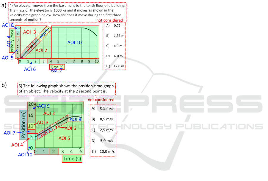
3.5 Position and Size of AOIs
Figure 1 shows the analyzed AOIs of item 4 (panel a)
and item 5 (panel b). In both problems, the analyzed
AOIs cover only the graphical area because we are in-
terested in the visual problem-solving strategy of the
students and the prediction probability based on this
data. It was previously shown that the students who
choose the correct answer focus significantly longer
on this answer option than students who do not choose
an incorrect answer (Klein et al., 2019b). Therefore,
it is likely to have a strong effect on the prediction
probability of the algorithm when including this op-
tion and the performance of the algorithm could not
unambiguously be assigned to the problem-solving
strategy. We also did not include the text area in the
Classification of Students’ Conceptual Understanding in STEM Education using Their Visual Attention Distributions: A Comparison of
Three Machine-Learning Approaches
39
analysis because the total visit duration on the text is
likely to be attributed to reading speed which would
also cause a confusion with our focus on the graphical
problem-solving strategy of the students.
Item 4 addresses the area concept which needs to
be applied to extract information about the position
from the v(t) graph. One way to determine the area
of this graph in the first three seconds is that the y-
axis interval [0,4] is multiplied with the x-axis inter-
val [0, 3] and the result is divided by 2 since the graph
is linear and starts at the origin. Item 5 addresses the
Figure 1: Quantitative Items of the TUG-K Analyzed in
This Work Which Address the Area Concept in Item 4
(Panel a) and the Slope Concept in Item 5 (Panel B). AOIs
Which Exhibit a Significant Difference in the TVD between
Students with Correct and Incorrect Answers Are Labeled
in Red. Those AOI with an Insignificant Difference in the
TVD Are Labeled in Blue.
slope concept which needs to be applied to extract the
velocity from a x(t)- graph (where x(t) means the po-
sition of an object at time t.). Here, the graph does not
pass through the origin, so it is necessary to calculate
the fraction of the size of the y-axis interval [5,10] and
the size of the x-axis interval [0,2].
The position, orientation and size of AOIs are
motivated by the Information-Reduction Hypothesis
which states that experts visually select conceptual-
relevant areas more efficiently (Haider and Frensch,
1996) and the previous work by Klein et al. who
found that students which solve a problem correctly
focus longer on areas along the graph and on the axes
(Klein et al., 2019a).
In this line, we first isolated the point directly
mentioned in the question text, here ”the first three
seconds” (item 4) and ”the 2 second point” (item 5),
which we call the surface feature, and all areas which
are directly linked to it, which is the point on the graph
(item 4: x = 3, y = 4 (AOI 9); item 5: x = 2, y = 10
(AOI 6);) and the associated point on the y-axis (item
4: y = 4 (no label); item 5: y = 10 (AOI 3)). There-
fore, we separated the area along the linear part of the
graph into two (item 4) and three (item 5) sections
in order to isolate the area that is directly related to
the surface feature. Additionally, we selected the end
point of one possible y-axis interval y = 5 (AOI4 in
item 5). The remaining areas along the axes, around
the graph and the axes labels are considered individu-
ally.
4 RESULTS
In Figure 1, the AOIs are ordered according to the
ascending order of p-values which result from the F-
statistics (see Table 1 and 2). Those AOIs in which
there is a significant relation of the response correct-
ness (coded as 1=correct and 0=incorrect) on the total
visit duration within the F-statistics are labeled in red
(significance level p < 0.05). In item 4, the answer
correctness exhibits a significant dependence on the
TVD in three AOIs, namely the lower section of the
graph (AOI 1), the area underneath the graph (AOI 2)
and the area above the graph (AOI 3).
In item 5, the answer correctness is also signifi-
cantly related to the lower graph section (AOI 1) as
well as the area underneath (AOI 5) and above the
graph (AOI 2). Additionally, there is a significant dif-
ference in the TVD between students who gave a cor-
rect and an incorrect answer in the areas around the
points on the y-axis y = 5 (AOI 4) and y = 10 (AOI
5) and the point on the graph (AOI 6: x = 2, y = 10)
which is linked to the surface feature.
Overall, in both items, the surface feature does not
show a significant difference in the TVD between stu-
dents with correct and incorrect answers but the lower
graph area and the areas below and above the graph
indeed shows a significant difference in the TVD be-
tween students with correct and incorrect answers.
The statistical difference in the TVD between stu-
dents who gave a correct and an incorrect answer is
also visible in the heat map of the relative attention
duration in Figure 2. In comparison of the total visit
duration in item 4 between students who answered
CSEDU 2020 - 12th International Conference on Computer Supported Education
40
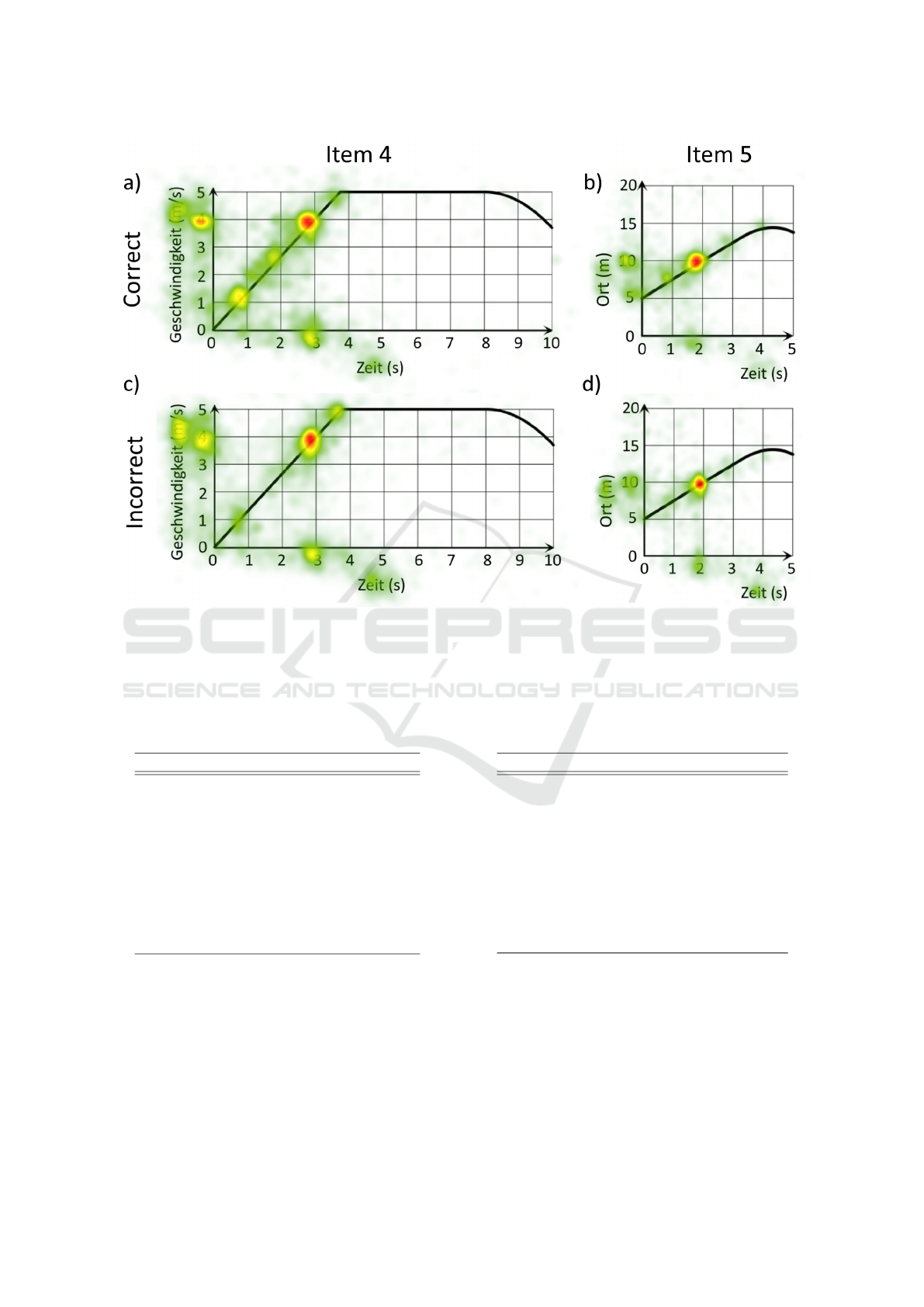
Figure 2: Heat Maps of the Relative Attention Duration for Item 4 (Left Panels) and 5 (Right Panels) for Students Who
Answered Correctly (Top Panels) and Students Who Answered Incorrectly (Bottom Panel).
Table 1: AOIs of Item 4 including the Statistical Compar-
ison (Effect Size in Terms of the p-Value) of the TVD be-
tween Students Who Answered Correctly and Those Who
Answered Incorrectly for Each AOI. The First Three AOIs
Are below the Significance Level of p < 0.05.
Area p-value Label
Lower graph section < 10
−4
AOI 1
Below graph 0.0083 AOI 2
Above graph 0.0163 AOI 3
y-axis label 0.3677 AOI 4
y-axis interval: [0, 3] 0.4109 AOI 5
x-axis interval: [0, 2] 0.4409 AOI 6
x-axis label 0.4919 AOI 7
y-value: y = 5 0.5672 AOI 8
Upper graph section 0.6301 AOI 9
Remaining graph area 0.6474 AOI 10
this question correctly (panel a) and those who an-
swered it incorrectly (panel b), it is noticeable that
students with a correct answer pay more visual at-
tention on the lower section of the linear part of the
graph as well as below the graph and the y-axis tick
labels for y < 4. In contrast, students with an incor-
rect answer allocate more relative attention to the end
of the linear region and the units of the y-axis. In this
illustration, it seems that both student groups focus
Table 2: AOIs of Item 5 including the Statistical Compar-
ison (Effect Size in Terms of the p-Value) of the TVD be-
tween Students Who Answered Correctly and Those Who
Answered Incorrectly for Each AOI. The First Six AOIs Are
below the Significance Level of p < 0.05.
Area p-value Label
Lower graph section 0.0002 AOI 1
Above graph 0.0006 AOI 2
y-value: y = 10 0.0046 AOI 3
y-value: y = 5 0.0117 AOI 4
Below graph 0.0387 AOI 5
Point: x = 2, y = 10 0.0453 AOI 6
y-value: y = 7.5 0.2086 AOI 7
Non-linear part 0.2098 AOI 8
y-axis interval: [15, 20] 0.3791 AOI 9
y-value: y = 0 0.4227 AOI 10
similarly on the surface feature (x = 3) and the areas
which are linked to the surface feature, i.e. the point
(x = 3, y = 4) and yaxis tick label y = 4.
Similarly, the heat maps of the relative durations
of item 5 show that the students who gave a correct
answer (Figure 2b) seem to focus on distinct points
on the graph where the graph intersects with the ver-
tical grid lines whereas the students with an incorrect
answer (Figure 2b) show a more scattered visual at-
Classification of Students’ Conceptual Understanding in STEM Education using Their Visual Attention Distributions: A Comparison of
Three Machine-Learning Approaches
41
tention. In this way, it is visible that students with
a correct answer focus longer on the lower section of
the graph and on the y-axis tick value y = 5. Contrary,
students who gave an incorrect answer seem to focus
more on the x-axis and y-axis labels. It seems that
above the graph, there is a particular difference in the
area between the graph and the y-axis for 5 < y < 10.
Comparably to item 4, in item 5, both student groups
seem to pay a similar amount of visual attention to
the surface feature (x = 2) and the areas which are
linked to it ((x = 2, y = 10) and y = 10). To ana-
0.0 0.2 0.4 0.6 0.8 1.0
0.5 0.6 0.7 0.8 0.9
Item 4: 4 Features
Testing set size
Prediction Probability
SVM
RF
MLP
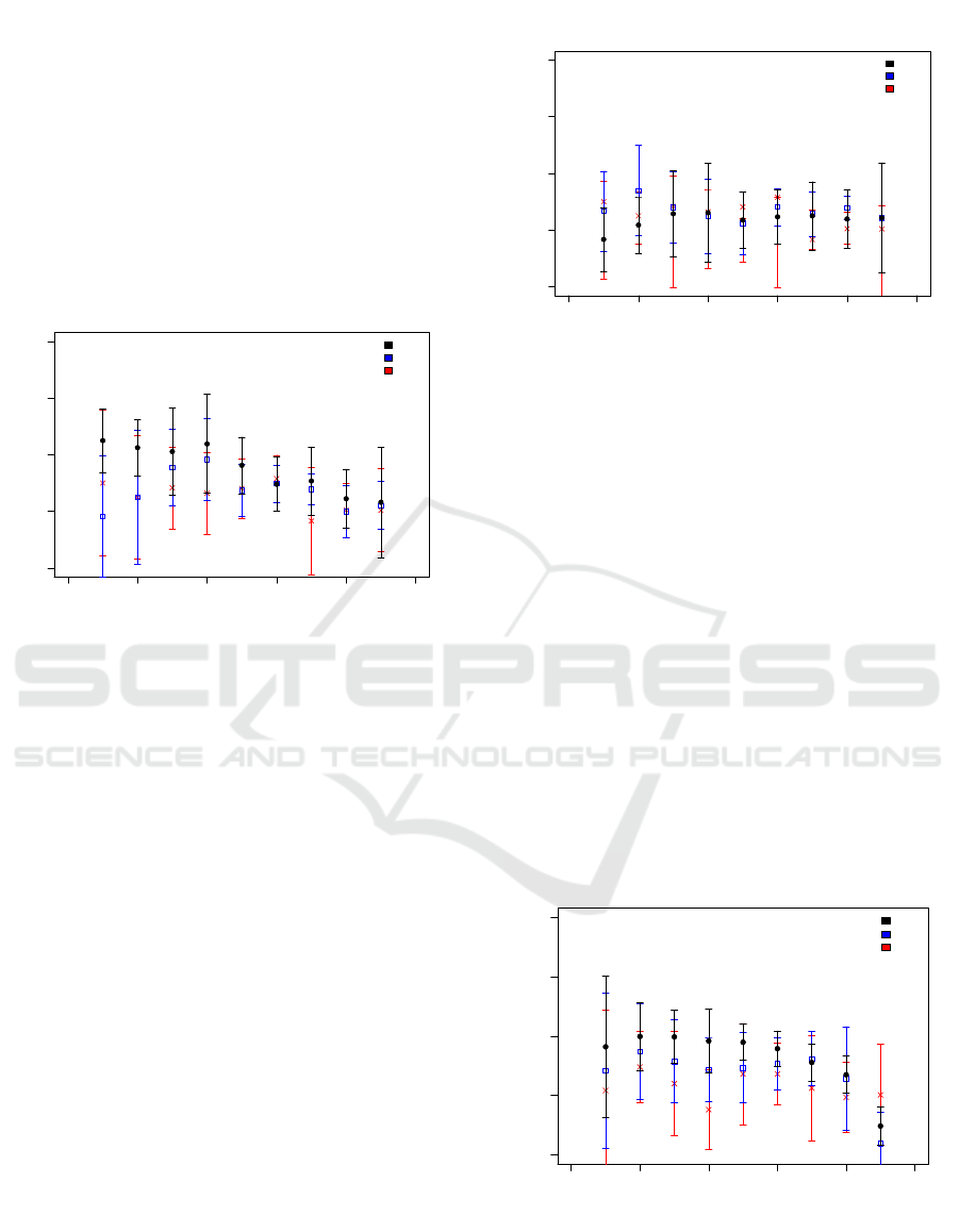
Figure 3: Probability of a Correct Prediction of Three Dif-
ferent Machine Learning Algorithms for the Response Cor-
rectness of Item 4 as a Function of Test Set Size for 4 Fea-
tures. The Data Points Represent the Average of 10 Inde-
pendent Runs and the Error Bars Reflect the Standard De-
viation of These Runs.
lyze the predictability of the identified AOIs in the
item 4, addressing the area concept, and item 5, tar-
geting the slope concept, we trained three different
algorithms with different number of features. Figure
3 displays the performance of the three algorithms us-
ing a small number of features. In this case, the best
performance among three, four and five features were
obtained when using four features. Please keep in
mind that the training set and the test set are disjoint
data sets. This means that the training set size is 1− x
(where x is the testing set size).
In Figure 3, it is noticeable that the prediction
probability of the SVM is increasing with test set sizes
(i.e. with decreasing training set sizes) whereas the
MLP remains unaffected by the change in test set size
within the error bars and the RF even exhibits a max-
imum at a testing set size of 0.4. At large test set
sizes (> 0.5), the prediction performance of the re-
sponse correctness of the three algorithms is more or
less comparable whereas the SVM exceeds the per-
formance of the other two algorithms at small test set
sizes.
0.0 0.2 0.4 0.6 0.8 1.0
0.5 0.6 0.7 0.8 0.9
Item 4: 9 Features
Testing set size
Prediction Probability
SVM
RF
MLP
Figure 4: Prediction Probability for the Response Correct-
ness of Item 4 as a Function of Test Set Size for 9 Features.
The Data Points Represent the Average of 10 Independent
Runs and the Error Bars Reflect the Standard Deviation of
These Runs.
Figure 4 shows the prediction probability of the
three algorithms using the TVD of 9 AOIs for testing
and training. Here, we show the results of 9 features
because it performs best among 8, 9 or 10 features for
testing and training and we intended to contrast the
algorithm’s performance for a small and large num-
ber of features. In comparison to 4 features, the per-
formance of the deep neural network (MLP) with 9
features is the same at small and at large test set sizes.
The prediction probability of the RF is comparable
between 4 and 9 features at large test set sizes (> 0.4)
and, at small test set sizes (< 0.3), it is enhanced. The
predictive power of the SVM also shows a similar per-
formance at large test set sizes (≥ 0.6) and a clearly
decreased performance at small test set sizes (≤ 0.5).
0.0 0.2 0.4 0.6 0.8 1.0
0.5 0.6 0.7 0.8 0.9
Item 5: 3 Features
Testing set size
Prediction Probability
SVM
RF
MLP
Figure 5: Prediction Probability for the Response Correct-
ness of Item 5 as a Function of Test Set Size for 3 Features.
As before, the Data Points Represent the Average of 10 In-
dependent Runs and the Error Bars Represent the Standard
Deviation of These Runs.
CSEDU 2020 - 12th International Conference on Computer Supported Education
42
0.0 0.2 0.4 0.6 0.8 1.0
0.5 0.6 0.7 0.8 0.9
Item 5: 10 Features
Test set size
Prediction Probability
SVM
RF
MLP
Figure 6: Prediction Probability for the Response Correct-
ness of Item 5 as a Function of Test Set Size for 10 Features.
As before, the Data Points Represent the Average of 10 In-
dependent Runs and the Error Bars Represent the Standard
Deviation of These Runs.
For item 5, we also selected the best performance
of the three algorithms to predict the response correct-
ness for a small number of features (here, the TVD of
3 AOIs) and a large number of features (the TVD of
10 AOIs). Figure 5 shows the probability of a cor-
rect prediction using three features. In this case, there
is a constant performance for the three algorithms for
small and medium test set sizes (< 0.7) and decreas-
ing trend of the SVM and RF with increasing test set
size for large test set sizes (≥ 0.7) whereas the MLP
remains constant. Among small and medium test set
sizes there is a similar hierarchy among the three al-
gorithms: The deep neural network shows the lowest
performance with a maximum performance of 65% at
a test set size of 0.2, the RF shows a higher predic-
tion probability at nearly all test set size and reaches
a maximum of 68% at a test set size of 0.2, and the
SVM outperforms the other two algorithms at small
and medium test set sizes with a maximum performs
of 70% at a test set size of 0.2. At large test set
sizes, the performance of the SVM and RF decrease
most strongly, even below the value of the MLP at the
largest test set size.
In comparison to 3 features, Figure 6 shows the
probability of a correct response prediction using 10
features. It is noticeable that the predictive power of
the MLP is most strongly decreased for all test set
sizes, so the performance difference in comparison
to the other two algorithms. Here, the performance
of the SVM got slightly reduced at nearly all test set
sizes except for the smallest test set size (). In con-
trast to the other algorithms, the performance of the
RF remains unaffected at nearly all test set size. De-
spite the changes in performance when increasing the
number of features, the performance of the SVM still
exceeds the performance of the other two algorithms
at small and medium test set sizes (≤ 0.6). At large
test set sizes the average prediction probability of the
RF is slightly higher than the one of the other two al-
gorithms.
5 DISCUSSION
In this work, we studied the probability of an accurate
prediction of students’ response correctness during
physics line-graph problems of three machine learn-
ing algorithms when trained by different eye-tracking
data sets. We analyzed the TVD as a measure of the
visual attention distribution during problem-solving
of physics line-graph items addressing the slope (item
5) and the area concept (item 4) from the TUG-K.
In item 4, we found that the TVD in three AOIs is
significantly higher for students with correct answers
in comparison to those with incorrect answers, which
is the lower graph area, the area underneath and above
the graph. This means that students which determine
the area underneath the graph correctly also focus
longer on this area. In this problem, there are sev-
eral ways to determine the area underneath the graph.
One way would be to calculate the area of the rectan-
gle (3s · 4m/s) and divide it by two, since the graph
is the diagonal in this rectangle. When applying this
strategy, it is not obvious why the students would fo-
cus longer on the area underneath or above the graph
because it does not contain procedure-relevant infor-
mation. Another way to determine the area would
be to count the squares underneath (or above) the
graph. This strategy, in fact, requires the student to
focus on this area in order to extract the number of
squares. At this point, we cannot unambiguously con-
clude which strategy the students apply who solved
this item correctly. To solve this open question and to
understand more about the relation between problem-
solving strategy and eye-tracking data, future research
needs to include students’ comments such as a retro-
spective think aloud study.
In item 5, we found that students who solve this
quantitative problem correctly also focus longer on
the lower graph area. This observation is in agreement
with Klein et al. who observed that students who
answer qualitative slope items correctly have more
fixations along the graph than students who give the
wrong answer (Klein et al., 2019a). In this item, stu-
dents also focus longer on the area underneath and
above the graph. In this case, we assume that it might
be a part of the slope determination. One approach
to calculate the slope is to mentally construct a right-
Classification of Students’ Conceptual Understanding in STEM Education using Their Visual Attention Distributions: A Comparison of
Three Machine-Learning Approaches
43

angled triangle underneath (or alternatively on top of)
the graph in the way that the hypotenuse is parallel to
the graph and the right-angled sides are parallel to the
axes. The slope results from the fraction of the right-
angled sides (∆y/∆x). The visual attention could be
attributed to the mental construction of this slope tri-
angle. Additionally, there is also a higher attention on
the specific points on the y-axis (y = 5 and y = 10).
These two points are the two most likely points to be
used as end points of an y-axis interval because only
at these two y-values the graph overlaps with an inter-
section of the grid.
Furthermore, we analyzed the probability of a cor-
rect prediction of the students’ response of three dif-
ferent algorithms. Overall, it is noticeable that the
SVM performs best in several of the cases, such as
at small numbers of features (4 features in item 4; 3
features in item 5) at small and medium test set size
(< 0.6) or performs as good as other algorithms, for
instance, at a small number of features (4 features in
item 4; 3 features in item 5) at large test set sizes
(> 0.6) or with 9 features in item 4 at medium to
large test set sizes (> 0.4). However, the SVM also
seems to have some weaknesses. When the number
of features increases, for instance in item 4 from 4 to
9 features or in item 5 from 3 to 10 and to 13 (see
Appendix) features, the performance of the SVM de-
creases noticeably at small test set sizes (in item 4)
and at medium test set sizes (in item 5). Similarly,
the performance of the deep neural network decreases
with increasing number of features. In contrast to
that, for the studied area and slope concept, the perfor-
mance of the RF seems to be the most consistent when
changing the number of features. Here, an increase in
the number of features means that there are features
added in which the TVDs in the AOIs do not exhibit
a significant difference between students who answer
correctly and incorrectly. It seems that this causes a
problem, particularly for the SVM and the MLP. The
performance of the RF is not affected when additional
features are added.
Here, we anticipate that an important factor which
causes the dependence of the algorithms on the num-
ber of features is the discriminatory power of the
features between students who answer correctly and
those who answer incorrectly. The creation of the
kernel-based multidimensional decision boundary in
the SVM seems to cause a better prediction than
the feature selection-process in the RF and weight-
adjustment process in the MLP when trained with dis-
criminating data. When including features with p-
values larger than 0.05, we found a decreasing per-
formance of the SVM. It seems that the creation of
the decision boundary is largely compromised when
including data which does not discriminate well. The
advantage of the RF here is that the algorithm selects
the relevant features and does not include unneces-
sary features. This explains why an increasing num-
ber of features, even adding non-discriminating fea-
tures does not seem to affect the performance of the
RF. This selection process also seems to outperform
the weight-adjusting process during the training of the
MLP.
In most of the cases, the algorithms show an in-
creasing trend with decreasing test set size. This
means, when the algorithms are trained with a larger
number of instances, the classification of the test set
improves. In those cases, the performance of the algo-
rithms would benefit from a larger number of training
instances. To optimize the performance of the algo-
rithms apart from using a larger number of training
data, one could, for instance, improve the feature se-
lection process, particularly with identifying and in-
cluding more features which show a significant dif-
ference between students with correct and incorrect
answers. Apart from that, one could include a dimen-
sionality reduction or optimize the impurity level in
the case of decision trees. However, the identification
of the optimal tree is a time consuming task (G
´
eron,
2019).
6 CONCLUSION
In this work, we used remote eye tracking to study
the visual strategies of students to solve physics line-
graph problems targeting the area and the slope con-
cept. We evaluated a large data set of 115 high school
students who solved the TUG-K and found that stu-
dents who solve an exemplary quantitative area prob-
lem correctly focus significantly longer on the area
along the graph, not only on areas which are linked
to the surface, and on the area underneath and above
the graph. This gaze behavior can be explained with
specific mathematical problem-solving strategies but
further research is required to support this hypothe-
sis. Similarly, students who solve a quantitative line-
graph problem addressing the area concept also pay
more visual attention to the area along the graph, un-
derneath and above the graph and, additionally, they
focus longer on specific points on the y-axis which are
likely to be end points of a y-axis interval.
Using a small and a large number of eye-tracking
features, we trained three different machine learning
algorithms to classify the students’ response correct-
ness. We found that in several cases the SVM ex-
hibits the best and the MLP shows the lowest perfor-
mance. However, we found that the performance of
CSEDU 2020 - 12th International Conference on Computer Supported Education
44

the SVM depends on the discriminatory power of the
features and the decreases if the algorithm is trained
with features which do not discriminate well between
students with correct and incorrect answers. In such
cases, the RF shows the most consistent performance
and reaches the same performance levels as the SVM
or even outperforms the SVM.
REFERENCES
Alemdag, E. and Cagiltay, K. (2018). A systematic review
of eye tracking research on multimedia learning. Com-
puters & Education, 125:413–428.
Beichner, R. J. (1993). Third misconceptions seminar pro-
ceedings (1993).
Beichner, R. J. (1994). Testing student interpretation of
kinematics graphs. American journal of Physics,
62(8):750–762.
Ceuppens, S., Bollen, L., Deprez, J., Dehaene, W., and
De Cock, M. (2019). 9th grade students’ under-
standing and strategies when solving x (t) problems
in 1d kinematics and y (x) problems in mathemat-
ics. Physical Review Physics Education Research,
15(1):010101.
Champagne, A. and Kouba, V. (1999). Written products
as performance measures. In Mintzes, J., Wandersee,
J., and Novak, J., editors, Assessing science under-
standing: A Human constructivist view, pages 224–
248. New York: Academic Press.
Forster, P. A. (2004). Graphing in physics: Processes and
sources of error in tertiary entrance examinations in
western australia. Research in science Education,
34(3):239–265.
Gegenfurtner, A., Lehtinen, E., and S
¨
alj
¨
o, R. (2011). Ex-
pertise differences in the comprehension of visualiza-
tions: A meta-analysis of eye-tracking research in pro-
fessional domains. Educational Psychology Review,
23(4):523–552.
G
´
eron, A. (2019). Hands-On Machine Learning with Scikit-
Learn, Keras, and TensorFlow: Concepts, Tools, and
Techniques to Build Intelligent Systems. O’Reilly Me-
dia.
Glazer, N. (2011). Challenges with graph interpretation: A
review of the literature. Studies in Science Education,
47(2):183–210.
Haider, H. and Frensch, P. A. (1996). The role of informa-
tion reduction in skill acquisition. Cognitive psychol-
ogy, 30(3):304–337.
Hoffman, J. E. and Subramaniam, B. (1995). The role of
visual attention in saccadic eye movements. Attention,
Perception, and Psychophysics, 57:787–795.
Ivanjek, L., Susac, A., Planinic, M., Andrasevic, A., and
Milin-Sipus, Z. (2016). Student reasoning about
graphs in different contexts. Physical Review Physics
Education Research, 12(1):010106.
Just, M. A. and Carpenter, P. (1976). Eye fixations and cog-
nitive processes. Cognitive Psychology, 8:441–480.
Kekule, M. (2014). Students’ approaches when dealing
with kinematics graphs explored by eye-tracking re-
search method. In Proceedings of the frontiers in
mathematics and science education research confer-
ence, FISER, pages 108–117.
Kekule, M. (2015). Students’ different approaches to solv-
ing problems from kinematics in respect of good
and poor performance. In International Conference
on Contemporary Issues in Education, ICCIE, pages
126–134.
Klein, P., K
¨
uchemann, S., Br
¨
uckner, S., Zlatkin-
Troitschanskaia, O., and Kuhn, J. (2019a). Student
understanding of graph slope and area under a curve:
A replication study comparing first-year physics and
economics students. Physical Review Physics Educa-
tion Research, 15(2):020116.
Klein, P., Lichtenberger, A., K
¨
uchemann, S., Becker, S.,
Kekule, M., Viiri, J., Baadte, C., Vaterlaus, A., and
Kuhn, J. (2019b). Visual attention while solving the
test of understanding graphs in kinematics: An eye-
tracking analysis. European Journal of Physics.
Klein, P., Viiri, J., Mozaffari, S., Dengel, A., and Kuhn, J.
(2018). Instruction-based clinical eye-tracking study
on the visual interpretation of divergence: How do
students look at vector field plots? Physical Review
Physics Education Research, 14(1):010116.
Kozhevnikov, M., Motes, M. A., and Hegarty, M. (2007).
Spatial visualization in physics problem solving. Cog-
nitive science, 31(4):549–579.
K
¨
uchemann, S., Klein, P., Fouckhardt, H., Gr
¨
ober, S., and
Kuhn, J. (2019). Improving students’ understanding
of rotating frames of reference using videos from dif-
ferent perspectives. arXiv preprint arXiv:1902.10216.
Kustov, A. A. and Robinson, D. L. (1996). Shared neural
control of attentional shifts and eye movements. Na-
ture, 384(6604):74.
LeCompte, M. D. and Preissle, J. (1993). Ethnography and
qualitative design in educational research. San Diego,
California: Academic Press.
Madsen, A. M., Larson, A. M., Loschky, L. C., and Re-
bello, N. S. (2012). Differences in visual attention
between those who correctly and incorrectly answer
physics problems. Physical Review Special Topics-
Physics Education Research, 8(1):010122.
Mayer, R. E. (2009). Multimedia learning. New York:
Cambridge University Press, 2 edition.
McDermott, L. C., Rosenquist, M. L., and Van Zee, E. H.
(1987). Student difficulties in connecting graphs and
physics: Examples from kinematics. American Jour-
nal of Physics, 55(6):503–513.
Posner, G. J., Strike, K. A., Hewson, P. W., and Gertzog,
W. A. (1982). Accommodation of a scientific concep-
tion: Toward a theory of conceptual change. Science
education, 66(2):211–222.
Rayner, K. (1998). Eye movements in reading and informa-
tion processing: 20 years of research. Psychological
bulletin, 124(3):372.
Rayner, K. (2009). Eye movements and attention in read-
ing, scene perception, and visual search. The quar-
Classification of Students’ Conceptual Understanding in STEM Education using Their Visual Attention Distributions: A Comparison of
Three Machine-Learning Approaches
45
terly journal of experimental psychology, 62(8):1457–
1506.
Salvucci, D. D. and Anderson, J. R. (2001). Automated
eye-movement protocol analysis. Human-Computer
Interaction, 16:39–86.
Scheiter, K., Schubert, C., Sch
¨
uler, A., Schmidt, H., Zim-
mermann, G., Wassermann, B., Krebs, M.-C., and
Eder, T. (2019). Adaptive multimedia: Using gaze-
contingent instructional guidance to provide person-
alized processing support. Computers & Education,
139:31–47.
Schnotz, W., V. S. and Carretero, M. (1999). New perspec-
tives on conceptual change. Pergamon.
Sch
¨
uler, A. (2017). Investigating gaze behavior during pro-
cessing of inconsistent text-picture information: Ev-
idence for text-picture integration. Learning and In-
struction, 49:218–231.
Susac, A., Bubic, A., Kazotti, E., Planinic, M., and Pal-
movic, M. (2018). Student understanding of graph
slope and area under a graph: A comparison of
physics and nonphysics students. Physical Review
Physics Education Research, 14(2):020109.
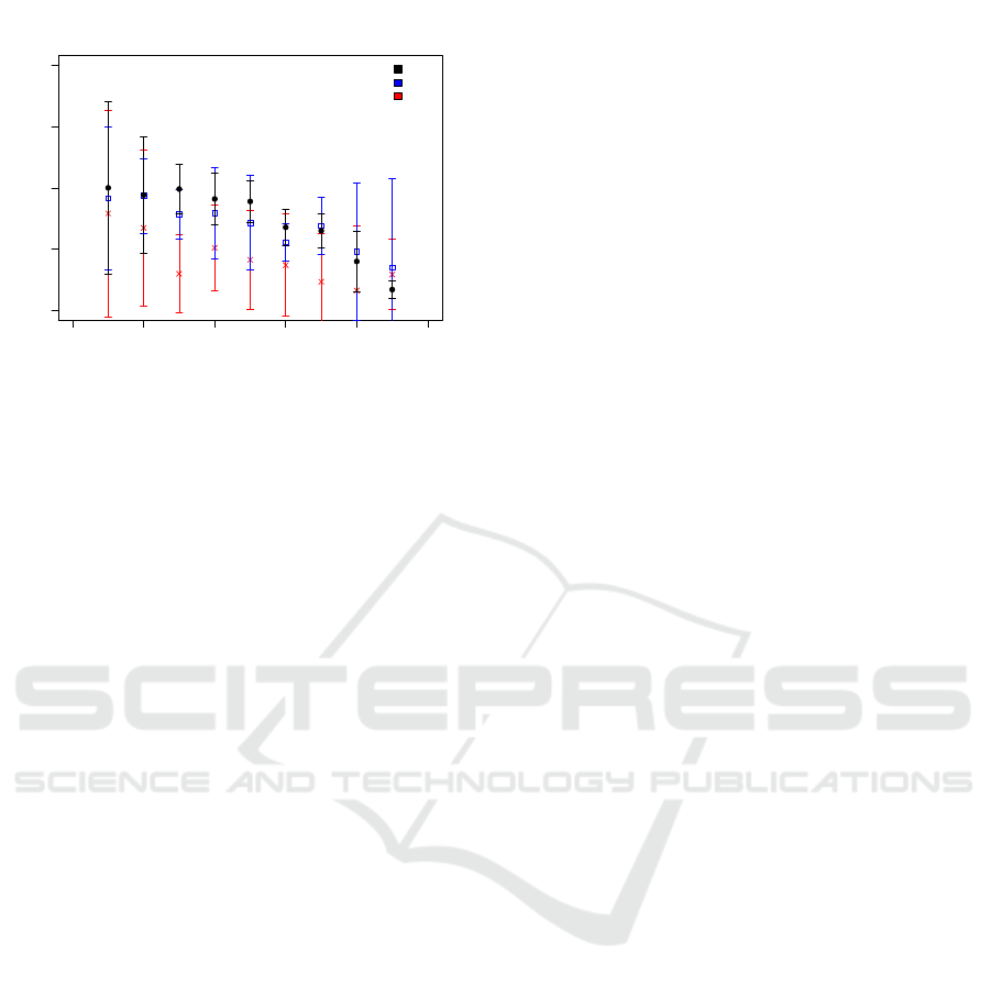
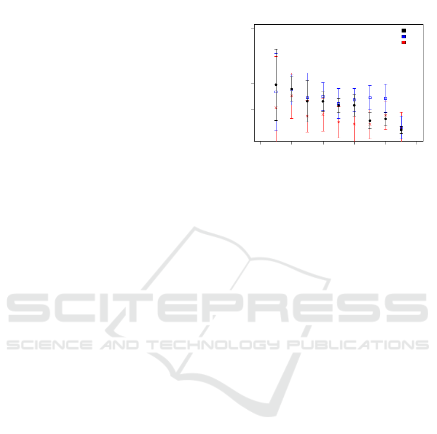
APPENDIX
Figure 7 shows the prediction probability for the re-
sponse correctness of the three algorithms for students
while solving item 5. In this case we used 13 fea-
tures for testing and training. It is noticeable that the
RF achieves the highest prediction probability at all
test set sizes except the smallest test set size. In com-
parison to the results with 3 and with 10 features the
prediction probability of the SVM has significantly
decreased, particularly at medium and large test set
sizes (≥ 0.3) so that it does not make the best predic-
tion anymore. At large test set sizes the SVM reaches
similar prediction probabilities as the MLP.
0.0 0.2 0.4 0.6 0.8 1.0
0.5 0.6 0.7 0.8 0.9
Item 5: 13 Features
Test set size
Prediction Probability
SVM
RF
MLP
Figure 7: Prediction Probability for the Response Correct-
ness of Item 5 as a Function of Test Set Size for 13 Features.
As before, the Data Points Represent the Average of 10 In-
dependent Runs and the Error Bars Represent the Standard
Deviation of These Runs.
CSEDU 2020 - 12th International Conference on Computer Supported Education
46
