Cognitive and Social Aspects of Visualization in Algorithm Learning

Lud

ek Ku

cera

1,2

Faculty of Mathematics and Physics, Charles University, Prague, Czech Republic

Faculty of Information Technologies, Czech Technical University, Prague, Czech Republic

Keywords:

Visualization, Algorithm, Invariant, JavaScript, Computer-supported Education, Social Aspect.

Abstract:

The present paper tries to point out two aspects of the computer supported education at the university level.

The ﬁrst aspect relates to cognition, in particular to methods of computer support of learning difﬁcult concepts

in natural sciences, computer science, and engineering, like mathematical notions and theorems, physical laws,

and complex algorithms and their behavior.

The second aspect is social - only few papers describe how the new educational methods are or have been

accepted by the community, whether they ﬁnished as a single experiment at the authors’ institution or whether

they are used in other schools, how difﬁcult is spreading them out and what kind of obstacles the authors meet.

We feel that even quite successful projects face certain inertia of the school system and the community of

teachers that make the wider use of new methods complicated.

1 INTRODUCTION

The present paper tries to point out two aspects of the

computer supported education at the university level

that are highly ignored in the mainstream of the ﬁeld.

The ﬁrst aspect relates to cognition, in particular

to methods of computer support of learning difﬁcult

concepts in natural sciences, computer science, and

engineering, like mathematical notions and theorems,

physical laws, and complex algorithms and their be-

havior.

The second aspect is social - only few papers de-

scribe how new educational methods are or have been

accepted by the community, whether they ﬁnished

as a single experiment at the authors’ institution or

whether they are used in other schools.

1.1 Knowledge and Skills

The ways of supporting education by computers relate

closely to the type of education. The goal of education

can be deﬁned as building knowledge and/or skills.

A skill is an ability to behave in certain way

to achieve required goals - e.g., manual skills in

medicine or social skills in management. Skills play

also very important role in arts.

For the purpose of the present paper, knowledge

is classiﬁed as soft and hard. We have no intension to

claim that one or the other type of knowledge is more

valuable.

One page of the proof of Farkas’ Lemma in the

Linear Programming Theory might take more time

the ten pages of a cardiology textbook, but no one

would claim that the mathematical knowledge is more

valuable than the medical one.

There is a very deep distinction between methods

of acquiring the soft and the hard knowledge that is

reﬂected in a rather pronounced way in methods of

computer support of such learnings.

Roughly speaking, the soft knowledge is often a

selection among possible worlds, based on a general

understanding of possibilities.

E.g., a heart is composed of several chambers, 2,

3, or 4. A cardiologist learns that a human hart has 4

chambers.

Examples of hard knowledge are abundant espe-

cially in natural sciences and engineering: e.g., prin-

ciples of magnetic resonance methods, quantum en-

tanglement, properties of smooth differentiability of

manifolds, and many others.

In its extreme form, acquiring hard knowledge is

trying to grasp the essence of one single situation,

which has no reﬂection in the previous learner’s ex-

perience. This implies that acquiring hard knowledge

is strictly different from acquiring the soft one.

Acquiring hard knowledge is a very important

(perhaps principal) part of education in many ﬁelds of

mathematics, computer science and natural sciences,

270

cera, L.

Cognitive and Social Aspects of Visualization in Algorithm Learning.

DOI: 10.5220/0009359102700277

In Proceedings of the 12th International Conference on Computer Supported Education (CSEDU 2020) - Volume 2, pages 270-277

ISBN: 978-989-758-417-6

but the inspection of the past years of CSEDU shows

there is practically no overlap with the research inter-

ests of the CSEDU community.

It seems that the main reason is sociological and

will be discussed later; the goal of the ﬁrst part of the

present paper is to induce interest of the community

in the exciting and important ﬁeld of ﬁnding methods

of computer support (usually visualization) for hard

knowledge learning.

1.1.1 Skills

There are many ways of computer support of manual

skill acquiring: videos showing proper ways of exe-

cution of desired operation, assembly, or other type of

manual activity; advanced computer games - e.g., the

paper Snyder et al. (2019) describes a serious game

RealTeeth, where dentistry students face virtual pa-

tients.

There are publications developing skills that aim

at a general evolution of personality of younger chil-

dren, e.g., Homanova and Havlaskova (2019).

Learning languages can also be classiﬁed as devel-

oping skills, with numerous articles describing vari-

ous systems of language learning computer support.

Building social skills can highly beneﬁt from us-

ing information technology. It is very frequent to use

electronic communication means to support commu-

nication among students in a group.

1.1.2 Soft Knowledge

The mainstream of the results in computer support

of education deals with building certain kinds of soft

knowledge. It is out of the scope of the present paper

to give a full review of different approaches that have

been published in the literature.

1.1.3 Hard Knowledge

The literature about ways of computer support of hard

knowledge acquiring is rather limited. We have found

no practically result of this type in the recent CSEDU

publications.

One of the reason why such results are so rare is

sociological and will be discussed later. Another pos-

sible reason is that methods of supporting skills and

soft knowledge learning systems are typically very

general, while a hard knowledge system is usually

directed to a single topic in a given narrow and ad-

vanced ﬁeld, and using an ad hoc approach that can

hardly be generalized.

Most of approaches widely used to support skills

and soft knowledge learning cannot be used in the

case of hard knowledge. Learning hard knowledge is

a single person activity, we are not aware of any sys-

tem that would use student collaboration to learn, e.g.,

the duality theorem of Linear Programming. Gaming

approach has also a very limited use.

We see the only way to use computers to support

hard knowledge learning - the method can be formu-

lated in a simple way, but its implementation is usu-

ally extremely difﬁcult: transform a mental process

that had lead the discoverer of a theorem, law, or an

algorithm to his discovery into a visual form that can

be shown in the computer screen.

It is important to note that this does not mean cre-

ating a visual representation of the publication de-

scription of the result; it is crucial that the discoverer’s

intuition and the ideas that are behind the discovery

are visualized in some form.

Nothing general can be said about the process,

each particular theorem, natural law or algorithm has

its own intellectual story, and it seems impossible to

ﬁnd any common feature that could be used to build a

more universal system.

2 PRINCIPLES OF SUPPORT OF

HARD KNOWLEDGE

LEARNING BY

VISUALIZATION

During the prenatal phase of a new human being, she

or she follows in some sense stages of development

of the mankind during past hundreds of thousands of

years. Similarly, when a learner tries to understand

difﬁcult concept, she or he has to follow in a certain

way the mental process that has led to the discovery of

the concept. As a conclusion, a computer support of

such a learning process should help a student to ﬁnd

and follow such a process.

The absence of such a feature is very frequent

source of a failure of a computer supporting system.

When a path leading to a discovery (which might

be a new mathematical theorem, computational algo-

rithm, or a newly formulated law of physics) has been

found, looking back to a series of failed attempts and

dead ends usually discloses that the path can be im-

proved, made shorter, the proof of the theorem made

simpler, certain unnecessary computations of an algo-

rithm eliminated, the evidence of a physical law made

more convincing.

A sometimes long series of improvements eventu-

ally gives a publication form of the description of the

new discovery which, quite often, is dead in the sense

that almost all traces of the intuition that lead to the

discovery are hidden and invisible. Mechanical ver-

Cognitive and Social Aspects of Visualization in Algorithm Learning

271

iﬁcation of statements demonstrating the correctness

can show that the result is valid, but it does not give

the true understanding.

An expert in the ﬁeld usually shares at least a part

of the intuition of the discoverer, and is able to see the

full landscape of a new discovery when given just few

hints and the static description involved in the publi-

cation text.

However, a novice in the ﬁeld must be guided and

the path that lead to the discovery and the discov-

erer’s view of the problem must be at least partially

disclosed to a learner to give her or him the full, ﬂex-

ible and long lasting knowledge.

Quite often, the discoverer’s intuition has a form

of images - sometimes mental images, in other cases

drawings on pieces of paper (or in sand in the case

of Archimedes). An author of a computer support-

ing system has to collect such images or to infer how

they could have looked, and then put them into screen.

Once again, let us note that only a small part of such

visual ideas eventually appear in the ﬁnal publication.

3 ALGORITHM LEARNING

3.1 Invariant Visualization

In this paper, hard knowledge learning is exempliﬁed

in the ﬁeld of algorithm learning by a system of visu-

alizations called Algovision algovision (2020). Some

of algorithms are quite complicated and a lot of men-

tal energy is necessary to understand them properly.

The ﬁeld of algorithms has one speciﬁc feature

that simpliﬁes our attempts to illustrate not only how

the algorithm works, but also why it has been designed

in the present form, and why the algorithm fulﬁlls its

task correctly.

In the case of a more complicated algorithm, it is

necessary to prove its correctness, i.e., to show that

it is able to achieve the desired output or result in all

cases. Our need for such proofs in not only the philo-

sophical one (in such a case we speak about Program

Correctness Theory), but also the practical one - we

have to give a guarantee that a real computer program

is ready for practical use (in such a case we speak

about Software Veriﬁcation).

However, the underlying method is the same in

both cases: we have to ﬁnd an invariant of the algo-

rithm - a logical statement such that

• it is veriﬁed at the beginning of the computation

under assumption the a valid input data were pro-

vided;

• the invariant together with conditions that induce

the end of the computation imply that the ﬁnal re-

sult veriﬁes all required conditions; and

• no single step of the computation violates the va-

lidity of the invariant.

Checking that an invariant of a given algorithm

satisﬁes all the above requirements is sometimes very

time consuming, but mechanical task. Some au-

tomatic software veriﬁcation systems perform such

checks automatically.

However, ﬁnding a full collection of invariants of

a given algorithm is a task that is far from being me-

chanical (it is possible to prove that ﬁnding an invari-

ant of a given algorithm is not an algorithmically solv-

able problem). The only way to such a statement is

using the discoverer’s intuition and understanding the

problem, as it has been discussed above.

We strongly believe (and share this belief with

many computer scientists) that knowing the invari-

ant is equivalent to understanding the algorithm. The

one who understands the algorithm knows internal re-

lations among variables of the program, and simply

writes them down to get the desired invariant. On the

other hand, the invariant simply writes what are our

goals in the actions the algorithm does, and this im-

plies the understanding of the method.

If we accept the postulate that the algorithm un-

derstanding is equivalent to the knowledge of the al-

gorithm invariant, educational algorithm visualization

becomes easier. The goal is not only to visualize the

data and to show them changing, but we have to ar-

range the data and possibly add some other visual ob-

jects to visualize the invariant(s). Since it often hap-

pens that relatively similar algorithms have quite dif-

ferent invariants (e.g., the shortest path algorithms of

Dijkstra and Bellman-Ford, see below), there is no

general method of visualizing algorithm invariants,

and any such animation is unique and incomparable

with the others.

3.2 Case Studies

The next subsections describe some of the visualiza-

tions of our system, pointing out the invariants and/or

ideas that support efﬁcient and easier learning of the

corresponding computational method.

3.2.1 Binomial Heap

The main idea of the binomial heap Vuillemin (1978)

is that it closely follows addition of binary numbers,

where “1” in the k-th column is represented by a tree

with 2

nodes. Visualization of the binomial heap

data structure can be found, e.g., at Galles (2020a),

CSEDU 2020 - 12th International Conference on Computer Supported Education

272

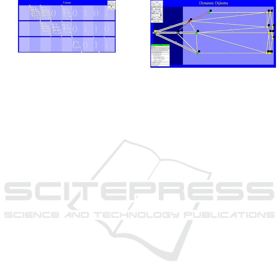
Figure 1: Binomial heap join as a binary number addition.

but only Algovision suggests immediately in a clear

way the correspondence with the original idea of J.

Vuillemin, see Fig. 1, where binary addition is pre-

sented in the background.

3.2.2 Fibonacci Heap

Visualization of the Fibonacci heap data structure

Fredman and Tarjan (1987) can be found, e.g., at

Galles (2020c). A student familiar with a binomial

heap has usually no problems with operations.

However, the form of Fibonacci heap trees is vari-

able, and the main property of the heap that a student

should learn in order to fully understand the heap and

the reason why it was invented is that a tree with large

root degree d must be large (in fact, the minimum size

of such a tree is F

, the d-th Fibonacci number - this

explains the name of the heap).

No attempt to illustrate this implication is made in

the above cited visualizations. On the other hand, the

principal part of our visualization is a series of play

scenes, where a student is given a sequence of tasks to

build trees of the form that appears in the background.

The tasks gradually lead a student to a surprising con-

clusion that is possible to build a large tree with a

small root degree, but not a small tree with a large

root degree.

Thus, in certain situations, a play-to-learn concept

can be used for hard knowledge acquiring as well.

3.2.3 Shortest Path Algorithms

Shortest path algorithms are usually the most ad-

vanced topic that is explained in a generic Algorithm

and Data Structure course at Computer Science de-

partments of Engineering Schools. Two of the main

algorithms of the class are algorithms of Dijkstra and

Bellman-Ford. They are very similar, the only dif-

ference being that the former uses a priority queue

to store open nodes of a graph, and requires non-

negative lengths of edges, while the other uses a sim-

ple queue and has no restrictions to edge labeling.

Since they are so similar, their visualizations

available on the web (e.g., Makohon et al. (2016);

Galles (2020b) as a selection of very large choice)

Figure 2: Dijkstra’s algorithm with horizontally moving

nodes.

look very similar as well. And this is wrong from the

point of view of understanding their behaviors that are

very different and this behavioral difference is what a

student has to know in order to understand well the

topic.

The background understanding of the algorithms

dictates two different visualization methods in our

collection:

In the Dijkstra visualization, nodes “slide” hori-

zontally and the x-coordinate of their location is pro-

portional to the estimation of their distance from the

origin, which is continuously upgraded by the algo-

rithm, see Fig. 2 (where nodes in a cluster near the

right side of the window are assumed to be yet in the

inﬁnite distance from the origin).

This arrangement is one of the most successful

applications of the rule that important values should

not be visualized as numbers (as it is done in the im-

plementations cited above), but by some geometrical

property (e.g., the height of a column, the width or the

shape of a certain visual object, or the location as in

the present case).

In a preliminary experiment with 14 students 2

weeks before Dijkstra’s algorithm was read in their

Algorithms and Data Structure class, a generic ani-

mation as cited above has been shown ﬁrst, followed

by our dynamic visualization.

The general comparison score average from the

range 1-10, where

“1=without dynamic visualization, I would have no

idea how it works”; and

10=“the dynamic version did not help at all”;

was 1.76 (including one student that admitted to give

a bad score because he knew the algorithm from his

high school), which we view as a conﬁrmation of our

design philosophy.

A new experiment with larger group of students

and electronic collection of their answers is prepared

for February 2020, and the results will be reported in

the full version of the paper.

On the other hand, our visualization of the Bell-

Cognitive and Social Aspects of Visualization in Algorithm Learning

273

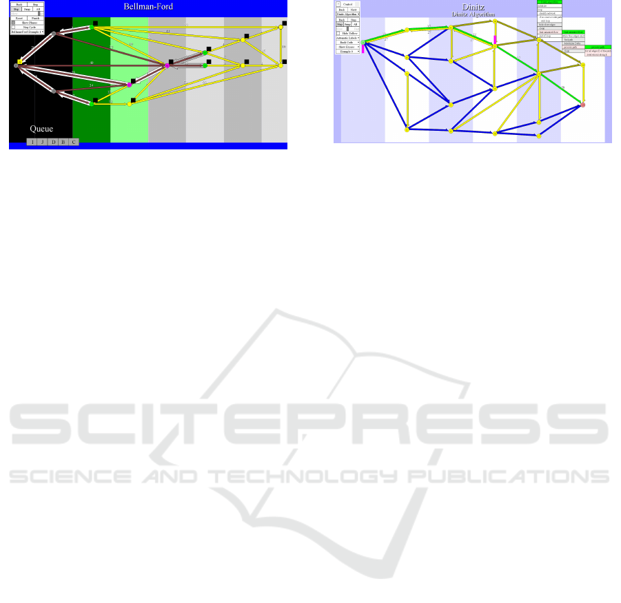
Figure 3: Bellman-Ford algorithm with phases.

man Ford algorithm is of the type “If I knew it, I

would not . . .”. After the computation is ﬁnished,

possibly without animation, nodes are partitioned ac-

cording to their distance from the origin in the tree

of shortest paths (represented by the wide white or

gray right-to-left oriented arrows behind the yellow

or brown edges of the original graph), see Fig. 3.

Unlike with the Dijkstra’s algorithm, in the

method of Bellman and Ford an already closed ver-

tex could be reopened when its estimation of the dis-

tance from origin changes, and all work previously

done with the work is invalidated. This makes the

time analysis of the algorithm especially involved.

In our representation, a student clearly sees that

• the black area on the left is already “dead”, all

variables have their ﬁnal values and no activity oc-

curs;

• the nodes in the dark green layer have their ﬁnal

values that are propagated to the light green layer;

and

• any other activity is useless, because it will later

be invalidated, when the corresponding nodes are

reopened (but we see it only now, after the whole

computation has been ﬁnished and is only back-

analyzed).

The visualization clearly shows that in all cases

(if no negative cycle is present) there is always some

activity that pushes the computation to the end after

ﬁnishing at most as many phases as is the number of

nodes.

The standard visualizations, e.g., those cited

above, give no hint to the time analysis of the

Bellman-Ford algorithm.

3.2.4 Network Flows: Dinitz Type Algorithms

The ﬁrst algorithm to ﬁnd the maximum ﬂow in a net-

work is due to Ford and Fulkerson Ford and Fulkerson

(1956). Its main problem is that its computation might

take long time that cannot be limited by any function

of the number of vertices and edges of the network,

Figure 4: Dinitz network ﬂow algorithm with layered net-

work.

but it depends only of the relation of the capacities of

edges.

In the Ford-Fulkerson algorithm, generalized

edges that can be used to build ﬂow-augmenting

paths, are both eliminated and reopened during the

computation, which causes sometimes very long com-

putation.

An improved version of the algorithm, discov-

ered simultaneously in Dinitz (1970) and Edmonds

and Karp (1972), is an implementation of the Ford-

Fulkerson algorithm, when a ﬂow augmenting path

selected by the algorithm must always have the small-

est possible number of edges.

The fact that this simple enhancement guarantees

fast computation could seem to be a mystery, unless

the visual representation of the graph is changed to

show layers (deﬁned by the length of the shortest path

from the network source), see Fig. 4.

It is easy to see in this representation left-to-right

oriented edges that may be used by the Dinitz algo-

rithm are blue or green (the green ones forming a par-

ticular augmenting path), the yellow edges are not on

any shortest source-to-sink path and hence should not

be used.

The picture clearly shows that each time an aug-

menting path is processed, at least one blue edge dis-

appears, while the edges that are reopened are the

opposites of blue edges, thus being oriented right-to-

left, not belonging to any shortest source-sink path at

the moment, and hence forbidden by the Dinitz algo-

rithm.

This is how our visualization makes it obvious that

the Dinitz algorithm approaches the end of the com-

putation in a very straightforward manner. No such

hints can be found in visualization that are published

in the web.

3.2.5 Fast Fourier Transform

FFT (Fast Fourier Transform) is an efﬁcient algorithm

for computing the discrete version of the Fourier

Transform, a useful tool for spectral analysis of digital

CSEDU 2020 - 12th International Conference on Computer Supported Education

274

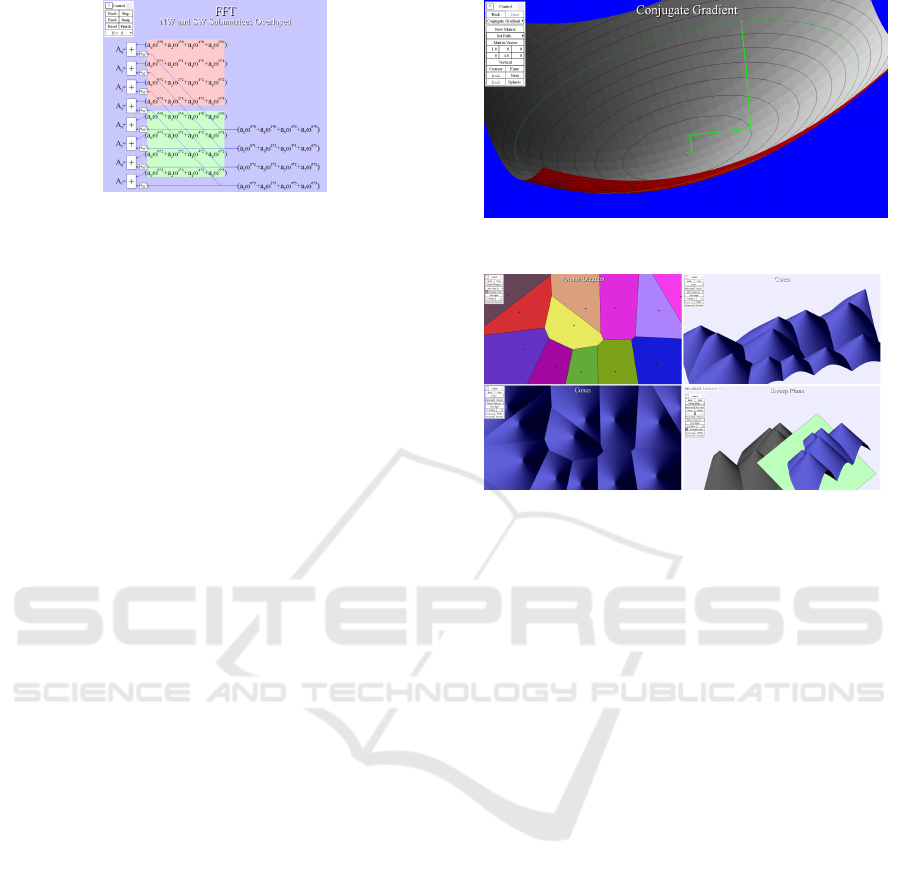
Figure 5: Explaining the FFT algorithm.

signals, data compression and other applications.

Our experience showed that high proportion of

students understood the method as the application of

the divide-and-conquer principle: partition the prob-

lem to two subproblems, solve them recursively, and

combined together.

In fact, the divide-and-conquer paradigm is really

used, but, since the matrix of the problem is two-

dimensional, there are four subproblems to be solved,

and the essence of the FFT analysis is that that there

are two pairs of identical subproblems.

This is one of our most successful visualizations,

because student examinations clearly showed a sub-

stantial drop of the percentage of students that misun-

derstood the FFT method in the way described above.

3.2.6 Conjugate Gradient Method

The CGM (Conjugate Gradient Method, Hestenes and

Stiefel (1952)) is the fundamental method of Numer-

ical Linear Algebra. The CGM and its more advance

variants (e.g., BiCGstab) are used in many applica-

tions like CFD (Computational Fluid Dynamic, which

covers virtual wind tunnels to test aerodynamics in

automotive and aerospace industry).

The problem of numerical solving systems of par-

tial differential equations that arise in physics and en-

gineering is reduced to sparse systems of linear equa-

tions, which in turn are solved as ﬁnding the mini-

mum of a quadratic functional given by the matrix of

the system. In Fig. 6 shows the situation in the 2-

dimensional case. The solution of the problem, repre-

sented by the red point at the bottom of the surface

is unknown, can be found by the Steepest Descent

method, which, however, needs many zig-zag itera-

tion.

The essence of the CGM Method is to shrink the

surface so that the horizontal elliptic contour lines be-

come circles. Then, the minimum is found as one it-

eration of the steepest descent.

Our experience shows that after having seen the

compression visualization of the notion of the con-

jugated gradient, students exhibit much better under-

standing of the CGM and higher ﬂexibility that makes

Figure 6: Steepest descent minimum ﬁnding.

Figure 7: Voronoi diagram.

them better prepared for applications of the CGM as

well as learning CGM generalizations.

3.2.7 Voronoi Diagram

With reference to Fig. 7, NW corner, given a ﬁnite

set of points of the plane (called sites, black dots

in the ﬁgure), we have to partition the plane so that

monochromatic areas around each site are collections

of all points of the plane, for which the site in the area

is the nearest site. The partition is called a Voronoi

diagram or a Dirichlet tessellation of the set of sites

(Dirichlet (1850); Voronoi (1908)).

Our visualization explains an elegant algorithm

due to Steve Fortune Fortune (1987). The key point

to understanding the algorithm is to imagine the plane

with sites inserted as a horizontal plane into the 3D

space; for each site, we also create a cone with its

summit in the site. A view of the obtained surface in

a general direction is in Fig. 7, NE corner. However,

if observed vertically, see Fig. 7, SW corner, the in-

tersections of cones reveal the boundary lines of the

Voronoi diagram.

The algorithm itself works by sweeping the moun-

tains of cones by an inclined plane (Fig. 7, SE corner).

The animation is one of the best examples of “Oh, I

see” visualization: with only a slight exaggeration,

since the moment students see the scene of the plane

sweeping the cones, most of them would be able to

write the corresponding program by themselves.

Cognitive and Social Aspects of Visualization in Algorithm Learning

275

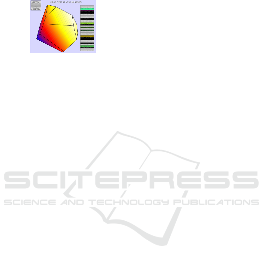
Figure 8: Simplex algorithm of Linear Programming in 3D.

3.2.8 Simplex Algorithm

The simplex algorithm, the oldest algorithm of Lin-

ear Programming, is still used frequently in practice.

For the history of the algorithm, see, e.g., Simplex

(2020). The way it is taught (especially outside Com-

puter Science, e.g., in schools of economy) is often

very formal and students just memorize certain com-

putational steps without having any understanding of

the principles of the method.

However, the problem and the algorithm have a

natural geometrical representation: the set of linear

inequalities deﬁnes a polytope in a space (see Fig. 8

taken from Algovision) A teacher or a learner can ro-

tate the polytope to see it from all directions. The

linear functional to be optimized is represented us-

ing colors of hot iron: dark blue for low values, light

yellow to white for high values. And the idea of the

simplex algorithm is to ﬁnd the hottest tip of the poly-

tope.

4 SOCIAL ASPECTS OF

COMPUTER SUPPORT OF

ALGORITHM LEARNING

A typical article in the ﬁeld of computer-supported

education presents motivation, a description of a par-

ticular supporting system, and a single example of us-

ing the system in education. This suggests that the

system has been used just in a single occasion by the

authors and no attempt was made to offer the system

to other educational institutions. Or, if the system is

successfully used in several schools, the social aspects

of the dissemination process are not mentioned.

It would also be interesting to know the distri-

bution of the expertise in the team of authors - such

an information might be valuable for those that start

working in the area of computed supported education

(and for experienced researchers as well).

4.1 The Golden Age of Algorithm

Animation and Its Decline

The temporal nature of algorithms immediately calls

for animated visualization. It was believed that the

universal paradigm is quite simple: take a static rep-

resentation of the background object of an algorithm

(usually a graph drawn in a textbook form or a se-

quence of numbers represented by columns of differ-

ent heights), and update them periodically as they are

updated by the algorithm. A continuous or step-by-

step update of the visual information is controlled in

a way that is well-known from programming develop-

ment system, when the option of interrupted “execu-

tion” of a program is used for debugging.

Some time ago, I had arrived to Pittsburgh the day

when Steelers played the Super-bowl ﬁnal, and it was

my strict obligation to see the match. Having no idea

of rules of football, I was even unable to ﬁgure out

who was winning (or how it happened that Steelers

won).

Unfortunately, the same situation occurred with

algorithm animations created using the above ap-

proach. A person with previous knowledge of an al-

gorithm was able to see clearly the progress of the

computation, but a novice student saw just a picture

changing in a messy and incomprehensible way, be-

ing usually unable to ﬁgure out what is going on.

The situation about 12 years ago was best charac-

terized by an article bassat Levy and Ben-Ari (2007)

with the title “We work so hard and they don’t use it:

acceptance of software tools by teachers”. Hardwork-

ing researchers were the authors of algorithm anima-

tions, “they” were teachers of algorithms at computer

science departments.

At the present time, the activity in algorithm ani-

mation and visualization has almost stopped; they are

certain sites that are mentioned in references that are

sometimes used as an illustration of algorithms, but

their use in the mainstream computer science teach-

ing is limited.

4.2 How to Offer a

Computer-supported Educational

System to Colleagues

With respect to the previous section, our experience is

rather different.

We have very good experience with accepting our

visualizations both by students and teachers. This

year, almost one third of computer science majors in

the ﬁrst year of their study at our university are taking

a facultative course based on Algovision in parallel

CSEDU 2020 - 12th International Conference on Computer Supported Education

276

with the standard and obligatory Algorithm and Data

Structure course using pdf slides.

While our colleagues from our university or even

abroad (including Stasko (2019)) are also quite en-

thusiastic with the way visualization of algorithms

and their background ideas makes learning easier and

more efﬁcient, when confronted with an offer to use

the visualization in their standard course, it seems that

they don’t hear a friendly offer, but they feel to be said

in a harsh voice “Hey, throw your stupid slides out of

window; what we offer is much better that you would

ever be able to do by yourself”.

Well, this is highly exaggerated, but if we try

to understand the point of view of an experienced

teacher with carefully prepared slides, who success-

fully teaches Algorithms and Data Structures already

for many years, we understand that it is in fact very

impolite and aggressive to try to make him or her to

throw away all his or her experience and to switch to

a completely different method.

The present paper has been prepared in a typeset-

ting system T

X. In one interview, its author, Don-

ald Knuth, mentioned his meeting with an owner of

a small publishing house, specialized in ﬁne typeset-

ting of mathematical books and journals. The pub-

lisher asked Knuth not to disseminate T

Xanymore,

because the system was destroying his tool of making

money to live. We are afraid that the reason why we

work so hard and they are not using it is very similar.

REFERENCES

algovision (2020). www.algovision.org, the main reference

to the visualization system presented in the paper.

bassat Levy, R. B. and Ben-Ari, M. (2007). We work so hard

and they don’t use it: acceptance of software tools by

teachers. In ITiCSE ’07: Proc. of 12th SIGCSE Conf.

on Innov. and Technol. in CS education, Dundee, Scot-

land. ACM Press.

Dinitz, Y. (1970). Algorithm for solution of a problem of

maximum ﬂow in a network with power estimations.

Dokl. Ak. Nauk SSSR, 11:1277–1280.

Dirichlet, G. L. (1850).

Uber die reduktion der positiven

quadratischen formen mit drei unbestimmten ganzen

zahlen. J. f

ur die Reine und Angewandte Math.,

40:209–227.

Edmonds, J. and Karp, R. M. (1972). Theoretical improve-

ments in algorithmic efﬁciency for network ﬂow prob-

lem. J. ACM, 19(2):248–264.

Ford, L. R. and Fulkerson, D. R. (1956). Maximal ﬂow

through a network. Canadian J. Math., 8:399–404.

Fortune, S. (1987). A sweepline algorithm for voronoi dia-

grams. Algorithmica, 2:153–174.

Fredman, M. L. and Tarjan, R. E. (1987). Fibonacci heaps

and their uses in improved network optimization algo-

rithms. J. ACM, 34(3):596–615.

Galles, D. (2020a). www.cs.usfca.edu/∼galles/visualization/

binomialqueue.html.

Galles, D. (2020b). www.cs.usfca.edu/∼galles/visualization/

dijkstra.html.

Galles, D. (2020c). www.cs.usfca.edu/∼galles/visualization/

ﬁbonacciheap.html.

Hestenes, M. R. and Stiefel, E. (1952). Methods of con-

jugate gradients for solving linear systems. J. Res.

National Bureau of Standards, 49(6):409.

Homanova, Z. and Havlaskova, T. (2019). Algorithmiza-

tion in a computer graphics environment. In CSEDU,

Heraklion, Crete, Greece, pages 466–473.

Makohon, I., Nguyen, D. T., Sosonkina, M., Shen, Y., and

Ng, M. (2016). Java based visualization and anima-

tion for teaching the dijkstra shortest path algorithm

in transportation networks. Int. J. Software Eng. &

Appl., 7(3):11–25.

Simplex (2020). en.wikipedia.org/wiki/simplex algorithm:

Simplex algorithm references.

Snyder, M., G

omez-Morantes, J., Parra, C., Carillo-Ramos,

A., Camacho, A., and Moreno, G. (2019). Devel-

opment of diagnostic skills in dentistry students us-

ing gamiﬁed virtual patients. In CSEDU, Heraklion,

Crete, Greece, pages 124–133.

Stasko, J. (2019). personal communication.

Voronoi, G. (1908). Nouvelles appliacations des param

etres

continus

a la the

eorie des formes quadratiques. J. f

die Reine und Angewandte Mathematik, 133:97–178.

Vuillemin, J. (1978). A data structure for manipulating pri-

ority queues. Comm. ACM, 21(4):309–315.

Cognitive and Social Aspects of Visualization in Algorithm Learning

277