
Hidden Markov Models for Pose Estimation
László Czúni and Amr M. Nagy
Department of Electrical Engineering and Information Systems, University of Pannonia,
Egyetem Street 10, Veszprém, Hungary
Keywords: Optical Object Recognition, Pose Estimation, Temporal Models, Hidden Markov Model, Deep Neural
Network.
Abstract: Estimation of the pose of objects is essential in order to interact with the real world in many applications such
as robotics, augmented reality or autonomous driving. The key challenges we must face in the recognition of
objects and their pose is due to the diversity of their visual appearance in addition to the complexity of the
environment, the variations of illumination, and possibilities of occlusions. We have previously shown that
Hidden Markov Models (HMMs) can improve the recognition of objects even with the help of weak object
classifiers if orientation information is also utilized during the recognition process. In this paper we describe
our first attempts when we apply HMMs to improve the pose selection of elementary convolutional neural
networks (CNNs).
1 INTRODUCTION
The recognition of 3D objects is an elementary
problem in many application fields such as robotics,
autonomous vehicles or augmented reality. However,
to interact with the objects of the environment, not
only specific or generic object recognition is
inevitable, but the determination of their pose is also
essential. Pose estimation is also a fundamental
problem in computer vision and large number of
algorithms have been proposed for the various
conditions and applications.
In recent years, the state of the art of convolutional
neural networks, like Regional CNN (Girshick,
Donahue, Darrell, & Malik, 2014), Fast R-CNN
(Redmon, Divvala, Girshick, & Farhadi, 2016), Mask
R-CNN (He, Gkioxari, Dollar, & Girshick, 2017),
(Redmon et al.,2016) and Single Shot Detectors (Liu
et al., 2016), have been proven to be very efficient for
object detection and recognition in RGB and depth
images, however these CNNs do not provide us
straightforward object pose estimation.
Similarly, the problem of the estimation of the 6-
DoF object pose was recently attacked by different
CNN approaches. Classical approaches can be
grouped ( Nöll, Pagani, & Stricker, 2011) as Direct
Linear Transformation, Perspective n-Point, and a
priori information estimators; they all suffer from the
problem of efficient feature selection,
correspondence generation and outlier filtering.
Contrary, CNN-based methods have the great
advantage to learn the combination of the best
possible features and classifiers or regressors.
Partially as a result of the Amazon Picking
Challenge (Correll et al., 2018), interest in object
manipulation has increased recently leading to the
development of several 6-DoF object estimation
methods. Many of these methods, such as PoseCNN
(Xiang, Schmidt, Narayanan, & Fox, 2018), SSD-6D
(Kehl, Manhardt, Tombari, Ilic, & Navab, 2017),
Real-Time Seamless Single Shot 6D Object Pose
Prediction (Tekin, Sinha, & Fua, 2018) and BB8 (Rad
& Lepetit, 2017), use convolution neural network
(CNNs) to estimate pose with high accuracy of
known objects in cluttered environments.
It is well-known that the general disadvantage of
neural network based methods is the dependency on
the training data and the utilized training methods.
For example, in (Xu, Bai, & Ghanem, n.d., 2019) the
performance drop caused by missing object labels is
analysed. Unfortunately, the generation of training
data is typically costly whether it is based on real or
syntactic data, especially if the pose is to be
represented (Rennie, Shome, Bekris, & De Souza,
2016).
We have previously shown that Hidden Markov
Models (HMMs) can improve the recognition of
objects from a sequence of images when weak object
classifiers are utilized (Czúni et al., 2017). Since our
598
Czúni, L. and Nagy, A.
Hidden Markov Models for Pose Estimation.
DOI: 10.5220/0009357505980603
In Proceedings of the 15th International Joint Conference on Computer Vision, Imaging and Computer Graphics Theory and Applications (VISIGRAPP 2020) - Volume 5: VISAPP, pages
598-603
ISBN: 978-989-758-402-2; ISSN: 2184-4321
Copyright
c
2022 by SCITEPRESS – Science and Technology Publications, Lda. All rights reserved

proposal utilized orientation sensors it is
straightforward to investigate whether it can improve
more sophisticated object recognizers (such as
CNNs) in pose estimation.
In this paper we show, that using a general object
classification network (namely VGG16), the
temporal inference generated by the HMM can
significantly increase the pose estimation
possibilities. The integration of our HMM approach
with more specific pose related networks is the task
of future.
In the following Section we shortly overview
some relevant papers then in Section 3 we describe
the details of our object pose estimation method. In
Section 4 our dataset and experiments are described
and finally in Section 5 we conclude our paper.
2 RELATED WORKS
6D object pose estimation methods can be
categorized roughly into feature-based, template-
based, and CNN-based methods.
Traditional local features (Collet, Martinez, &
Srinivasa, n.d, 2011.) utilize RGB images to extract
local keypoints and perform feature matching to
estimate the object pose. Local feature methods are
often fast and able to handle scene clutter and
occlusion, but the objects needed enough textures.
A 3D template model is built and used in
template-based methods (Hinterstoisser et al., 2013)
to scan various locations in the input image. A
similarity score is calculated at each position and the
best match is obtained by comparing these scores.
Template-based methods have great advantages on
texture-less objects however, they suffer from
occlusions.
In recent years, CNNs have started to dominate this
field either, so will review some of the most important
approaches.
A main concept behind PoseCNN (Xiang et al.,
2018) is to decouple the pose estimation into separate
components, allowing the network to identify the
dependencies and independence between them
explicitly. PoseCNN carries out three related tasks.
Starting from predicting an object label for each pixel
in the input image, estimating the 2D pixel
coordinates of the object, and estimating the 3D
Rotation by regressing convolutional features. There
are two levels in the network architecture of
PoseCNN. The first level is considered as the
backbone of the network consisting of 13 convolution
layers and 4 max pooling layers. Feature maps are
extracted with various resolution from the input
image. These features are spread across all the second
level tasks (i.e. semantic labelling, 3D translation
estimation, and 3D rotation regression) performed by
the network.
The SSD-6D (Kehl et al., 2017) approach is a
different method to detect instances of 3D objects and
estimate their 6D poses by a single shot from RGB
data only. It extends the common SSD paradigm to
cover the entire 6D pose space and these networks are
typically trained only on synthetic data. The network
produces six feature maps on multiple scales for each
input RGB image. To determine the object class, the
2D bounding box, and scores for possible viewpoints
and in-plane rotations, each map is convolved with
specifically trained kernels. After convolution, these
feature maps are analysed to create 6D pose
hypotheses. While SSD-6D can give very good
results it has its limitations, for example it is
necessary to find a suitable sampling of the viewing
space of the model to obtain the satisfactory results.
In the approach of (Sundermeyer, Marton,
Durner, & Triebel, 2019) augmented autoencoders
are used with single RGB images as inputs but
additionally depth maps may optionally be
incorporated to refine pose estimation. First SSD is
applied to detect the required object, to identify its
bounding box then Augmented Autoencoder (AAE)
is utilized to estimate the 3D orientation. Because the
Augmented Autoencoder is trained on 3D syntactic
models, they used a Domain Randomization (DR)
strategy to generalize from syntactic data to real.
3 THE PROPOSED METHOD
We follow the approach when a single CNN is to
recognize an object and its pose through several
observations then a statistical framework is applied to
evaluate the result of inferences and to make the final
object recognition and pose estimation. We have
chosen a well-known neural network, often used as a
backbone of more complex architectures, namely
VGG16 (Simonyan & Zisserman, 2015). We don’t
deal with the localization of the object within the
image frame. I. e. it gives no big stress for the
annotation procedure to generate training data but
makes it a hard work for the processing framework to
achieve good pose estimation.
In our view-centred representation, the outlook of
the object is modelled from different viewpoints with
multiple 2D images. It would be possible to make
these sample images from several elevations,
although in our experiments we implemented only a
Hidden Markov Models for Pose Estimation
599

single elevation methodology (since the used dataset
COIL contains only such data).
During the recognition consecutive queries, shots
taken from different viewing directions, are first
evaluated by VGG16 inference resulting in
confidence values. We assume that the relative pose
changes between the shots are recorded by easily
available IMU sensors (such as those built into most
mobile phone).
Using the image shots, the pre-built object
models, the trained VGG16 networks, and the change
in orientation between shots we use an HMM
framework to evaluate the image sequences and to
determine the most probable object and its pose series
generating the observations.
Since the order of sequential poses (the actual
changes of relative viewing directions) is determined
by the behaviour of the camera (or with other words
by the user) it cannot be generally modelled in the
model to determine the actual transition probabilities.
What we can do is to measure the real change in
relative poses query by query, with the help of IMU
sensors, and use geometric probabilities to evaluate
the chance of going from one state to another. For this
resolution of the problem of computing state
transitions, please see Subsection 3.2.
3.1 HMM Object Models
An HMM is defined by:
• its states S
i
,
• transition probabilities between states S
i
and S
j
(see Eq. 2),
• emission probabilities (P(o), see Eq. 7),
• initial state probabilities (π
i
).
To achieve object retrieval will need to build
HMM models for all elements of the set of objects
(M) where different poses (views made from different
orientations in our case) correspond to the states.
Then, based on the sequence of observations (o
i
), we
will find the most probable state sequence for all
object models. The state sequence among these,
which has the highest probability, will belong to the
object being recognized.
Traditionally, to build a Markov model means
learning its parameters (π, transition and emission
probabilities) by examining training examples.
However, our case is special: the probability of going
from one state to another severely depends on the
user’s behaviour and on the frame rate of the camera.
Thus, we can’t follow the traditional way, to use the
Baum-Welch algorithm for parameter estimation
based on several training samples but can directly
compute transition probabilities based on geometric
as described later. Observation probabilities will be
determined by the confidence values of the trained
CNN.
3.2 Object Poses as States in Hidden
Markov Models
Let S = {S
1
,…,S
N
} denote the set of N possible hidden
states of a model. In each step of an observation
process (denoted by index t) the model can be
described as being in one q
t
∈
S state, where t =
1,…,T.
In our approach the states can be considered as the
2D views (poses) of a given object model. This can
be easily imagined as a camera is targeting towards
and object from a given elevation and a given
azimuth. The number of possible states should be kept
low, otherwise the state transition matrix (A) would
contain too small numbers and finding the most
probable state sequence would be too uncertain. On
the other hand, small number of states would mean
that quite different appearances of objects should be
encoded by the same representation (now by a single
CNN for all objects and their poses) resulting in
decreased confidence again, thus the generation of
states should be designed carefully. In our
experiments we use static subdivision of the circle of
360º into 8º uniform sectors each with 45º opening.
We define the initial state probabilities π = {π
i
},
1≤i≤N based on the opening angle of the views:
π
=𝑃
(
𝑞
=𝑆
)
=
𝛼(𝑆
)
360
(1)
where α(S
i
) is the angle (given in degree) of
aperture of state S
i
.
3.3 State Transitions
Between two steps the model can undergo a change
of states according to a set of transition probabilities
associated with each state pairs. In general, the
transition probabilities are:
a
ij
= P(q
t
= S
j
|q
t−1
= S
i
) (2)
where now i and j indices refer to states of the HMM,
a
ij
≥ 0, and for a given state
∑
𝑎
,
=1 holds. The
transition probability matrix is denoted by A = {a
ij
},
1≤i,j≤N. The probability of going from one state to
another cannot be determined as part of the model but
we can directly compute transition probabilities based
on geometric probability as follows.
First define ∆
t−1,t
as the orientation difference
between two successive observations:
VISAPP 2020 - 15th International Conference on Computer Vision Theory and Applications
600
Δ
t
−
1,t
= α(o
t
) − α(o
t
−
1
)
(3)
Now define R
i
as the aperture interval angle
belonging to state S
i
by borderlines:
R
i
=[S
i
min
, S
i
max
) (4)
where S
i
min
and S
i
max
denotes the two (left and
right) terminal positions of state S
i
(one side is
specified with an open interval symbol). The back
projected aperture interval angle is the range of
orientation from where the previous observation
should originate:
.
(5)
Now, to estimate the transition probability we use
the geometrical probability concept applied on the
intersection of L
j
and R
j
:
𝑎
=𝑃𝑞
=𝑆
𝑞
=𝑆
=
∩
.
(6)
3.4 Recognition of Objects and Their
Poses
The emission probability of a particular observation
o
t
for state S
i
is defined as:
𝑏
(
𝑜
)
=𝑃
(
𝑜
|
𝑞
=𝑆
)
(7)
Applying VGG16 as a global object classifier, for all
poses of all objects, we can consider the confidence
values of inferences as b
i
-s. We assume that an
observation sequence contains only one class of
objects (possibly with several poses as the camera
moves on). Then for each possible object we
independently run the Viterbi algorithm to combine
the values of Eq. 2, Eq. 7, and π
i
-s to get the most
probable state sequences. Finally, we choose the
object with the highest probability value as the
recognized object and we can also determine the
poses selected for each query by the Viterbi path.
4 EVALUATION
4.1 Dataset
The COIL-100 dataset (Nene et al., 1996) includes
100 different objects each with 72 images taken by 5º
at the same elevation. We have chosen 40 objects
from the 100 for our experiments, see Fig. 1 for some
sample images. Each object was represented with 8
poses by equally divided sectors of 45º. Images are
originally with black background but to be more
realistic we have given different backgrounds,
selected from 200 random images, so the original
COIL images cover around 25% of the area of 128 ×
128 pixels (Fig. 1 bottom line). We believe that that
small adjacent black area around the objects does not
distort the results since it appears in all objects and
gives no advantage to the classifier. Thus, we got
2880 images (40 × 72) directly from COIL-100 and
11520 from augmentation. The dataset was cut into
training and testing parts so no queries of the
experiments could exactly match those images used
to train the CNN.
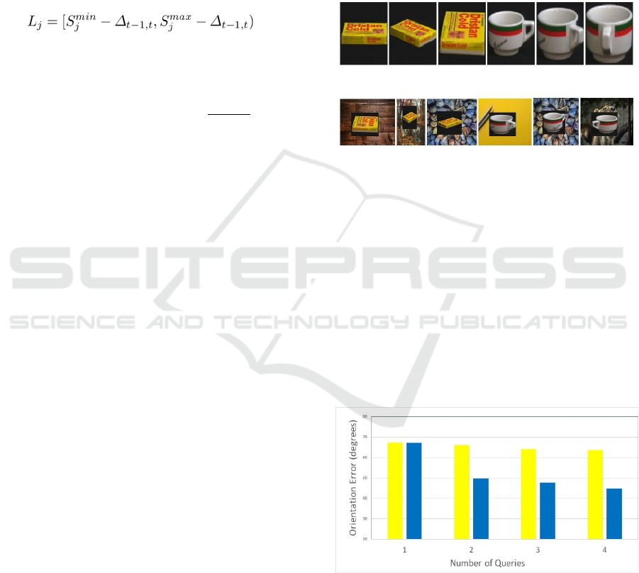
Figure 1: Top line: example objects from the COIL-100
dataset. Bottom line: test images with different
backgrounds.
4.2 Tests and Evaluations
A single VGG16 network was used to recognize all
320 (40 objects × 8 poses) classes. The network was
pre-trained with images of ImageNet (Russakovsky et
al., 2014). We did not refine the feature extraction
layers of the network, only the 4 end layers
responsible for classification, were replaced and re-
trained. During training image rotation, shift, shear,
zoom, and horizontal flip was applied as further
augmentation.
Figure 2: Average orientation error at different number of
queries for VGG16 only (yellow) and VGG+HMM (blue).
To get a general overview of the performance we
computed the pose error by averaging the orientation
error for each object and each pose estimated in 8
independent random experiments. As one could
expect the error may depend on the number of
Hidden Markov Models for Pose Estimation
601

observations (i.e. the number of queries). As Fig. 2
shows, increasing the number of queries results in the
decrease of average pose error from 67.18º to 44.78º.
As a reference, we computed the average error of the
VGG16 network illustrated by yellow in Fig. 2. These
values are ranging from 67.18º to 63.59º significantly
higher than the VGG+HMM technique. To highlight
the information added by the orientation sensor we
made tests where the transition probabilities were set
constant. This is named VGG+mHMM and shown by
green dotted lines in Fig. 2. There is no significant
difference between VGG16 and VGG+mHMM as
expected.
Interestingly, regarding the average object-level
recognition rate based on 4 queries, the VGG+HMM
method achieved 99.7% and the VGG16 resulted in
99.1%, which is a small difference thanks to the good
general recognition abilities of VGG16.
Figure 3: Average orientation error for each object, in case
of two queries, for VGG16 only (yellow), VGG+HMM
(blue), and VGG+mHMM with constant transition
probabilities (green dotted).
5 CONCLUSIONS
In our paper we discussed a probabilistic approach to
enhance the pose estimation capabilities of simple
classification networks such as VGG16. We utilized
the orientation sensor to estimate the transition
probabilities between poses thus HMMs could be
used to estimate the most probable pose sequences.
The improvement over the applied CNN is significant
as shown by experiments using 40 randomly chosen
objects of the COIL-100 dataset. In future we plan the
investigate how to fuse the model with more
sophisticated CNNs such as PoseCNN or SSD-6D.
ACKNOWLEDGEMENTS
We acknowledge the financial support of the
Széchenyi 2020 program under the project EFOP-
3.6.1-16-2016-00015, and the Hungarian Research Fund,
grant OTKA K 120367. We are grateful to the NVIDIA
Corporation for supporting our research with GPUs
obtained by the NVIDIA GPU Grant Program.
REFERENCES
Collet, A., Martinez, M., & Srinivasa, S. S. (2011). The
MOPED framework: Object recognition and pose
estimation for manipulation. International Journal of
Robotics Research, 30(10), 1284–1306.
Correll, N., Bekris, K. E., Berenson, D., Brock, O., Causo,
A., Hauser, K., … Wurman, P. R. (2018). Analysis and
observations from the first Amazon picking challenge.
IEEE Transactions on Automation Science and
Engineering, 15(1), 172–188.
Czúni, L., & Rashad, M. (2017). The Fusion of Optical and
Orientation Information in a Markovian Framework for
3D Object Retrieval. In International Conference on
Image Analysis and Processing, pp. 26–36.
Girshick, R., Donahue, J., Darrell, T., & Malik, J. (2014).
Rich feature hierarchies for accurate object detection
and semantic segmentation. Proceedings of the IEEE
Computer Society Conference on Computer Vision and
Pattern Recognition, 580–587.
He, K., Gkioxari, G., Dollar, P., & Girshick, R. (2017).
Mask R-CNN. Proceedings of the IEEE International
Conference on Computer Vision, 2980–2988.
Hinterstoisser, S., Holzer, S., Cagniart, C., Ilic, S.,
Konolige, K., Navab, N., & Lepetit, V. (2011).
Multimodal templates for real-time detection of
texture-less objects in heavily cluttered scenes.
Proceedings of the IEEE International Conference on
Computer Vision, 858–865.
Hinterstoisser, S., Lepetit, V., Ilic, S., Holzer, S., Bradski,
G., Konolige, K., & Navab, N. (2013). Model based
training, detection and pose estimation of texture-less
3D objects in heavily cluttered scenes. Lecture Notes in
Computer Science, 7724 LNCS(PART 1), 548–562.
Hodaň, T., Haluza, P., Obdrzalek, Š., Matas, J., Lourakis,
M., & Zabulis, X. (2017). T-LESS: An RGB-D dataset
for 6D pose estimation of texture-less objects.
Proceedings - 2017 IEEE Winter Conference on
Applications of Computer Vision, WACV 2017, 880–
888.
Kehl, W., Manhardt, F., Tombari, F., Ilic, S., & Navab, N.
(2017). SSD-6D: Making RGB-Based 3D Detection
and 6D Pose Estimation Great Again. Proceedings of
the IEEE International Conference on Computer
Vision, 1530–1538.
Liu, W., Anguelov, D., Erhan, D., Szegedy, C., Reed, S.,
Fu, C. Y., & Berg, A. C. (2016). SSD: Single shot
multibox detector. Lecture Notes in Computer Science
(Including Subseries Lecture Notes in Artificial
Intelligence and Lecture Notes in Bioinformatics), 9905
LNCS, 21–37.
Nöll, T., Pagani, A., & Stricker, D. (2011). Markerless
camera pose estimation - An overview. OpenAccess
VISAPP 2020 - 15th International Conference on Computer Vision Theory and Applications
602

Series in Informatics, 19, 45–54. In Visualization of
Large and Unstructured Data Sets-Applications in
Geospatial Planning, Modeling and Engineering (IRTG
1131 Workshop). Schloss Dagstuhl-Leibniz-Zentrum
fuer Informatik.
Rad, M., & Lepetit, V. (2017). BB8: A Scalable, Accurate,
Robust to Partial Occlusion Method for Predicting the
3D Poses of Challenging Objects without Using Depth.
Proceedings of the IEEE International Conference on
Computer Vision, 3848–3856.
Redmon, J., Divvala, S., Girshick, R., & Farhadi, A. (2016).
You only look once: Unified, real-time object detection.
Proceedings of the IEEE Computer Society Conference
on Computer Vision and Pattern Recognition, 779–788.
Ren, S., He, K., Girshick, R., & Sun, J. (2017). Faster R-
CNN: Towards Real-Time Object Detection with
Region Proposal Networks. IEEE Transactions on
Pattern Analysis and Machine Intelligence, 39(6),
1137–1149.
Rennie, C., Shome, R., Bekris, K. E., & De Souza, A. F.
(2016). A Dataset for Improved RGBD-Based Object
Detection and Pose Estimation for Warehouse Pick-
and-Place. IEEE Robotics and Automation Letters,
1(2), 1179–1185.
Russakovsky, O., Deng, J., Su, H., Krause, J., Satheesh, S.,
Ma, S., … Fei-Fei, L. (2014). ImageNet Large Scale
Visual Recognition Challenge.
Simonyan, K., & Zisserman, A. (2015). Very deep
convolutional networks for large-scale image
recognition. 3rd International Conference on Learning
Representations, ICLR 2015 - Conference Track
Proceedings. International Conference on Learning
Representations, ICLR.
Sundermeyer, M., Marton, Z. C., Durner, M., & Triebel, R.
(2019). Augmented Autoencoders: Implicit 3D
Orientation Learning for 6D Object Detection.
International Journal of Computer Vision, 11210
LNCS, 712–729.
Tejani, A., Tang, D., Kouskouridas, R., & Kim, T. K.
(2014). Latent-class Hough forests for 3D object
detection and pose estimation. Lecture Notes in
Computer Science (Including Subseries Lecture Notes
in Artificial Intelligence and Lecture Notes in
Bioinformatics), 8694 LNCS(PART 6), 462–477.
Springer Verlag.
Tekin, B., Sinha, S. N., & Fua, P. (2018). Real-Time
Seamless Single Shot 6D Object Pose Prediction.
Proceedings of the IEEE Computer Society Conference
on Computer Vision and Pattern Recognition, 292–301.
Xiang, Y., Schmidt, T., Narayanan, V., & Fox, D. (2018,
November 1). PoseCNN: A Convolutional Neural
Network for 6D Object Pose Estimation in Cluttered
Scenes.
Xu, M., Bai, Y., & Ghanem, B. (2019). Missing Labels in
Object Detection. CVPR Workshop. In The IEEE
Conference on Computer Vision and Pattern
Recognition (CVPR) Workshops
Nene, S.A., Nayar, S.K., Murase, H. (1996). Columbia
Object Image Library (COIL-100), Technical Report
CUCS, Department of Computer Science, Columbia
University, New York, NY, USA
Hidden Markov Models for Pose Estimation
603
