Mini V-Net: Depth Estimation from Single Indoor-Outdoor Images using

Strided-CNN

Ahmed J. Aﬁﬁ

1 a

, Olaf Hellwich

and Touﬁque Ahmed Soomro

2 b

Computer Vision and Remote Sensing, Technische Universit

at Berlin, Berlin, Germany

Electronic Engineering Department Quaid-e-Awam University of Engineering and Technology, Larkana Campus, Pakistan

Keywords:

Convolutional Neural Networks, CNN, Depth Estimation, Single View.

Abstract:

Depth estimation plays a vital role in many computer vision tasks including scene understanding and recon-

struction. However, it is an ill-posed problem when it comes to estimating the depth from a single view due

to the ambiguity and the lack of cues and prior knowledge. Proposed solutions so far estimate blurry depth

images with low resolutions. Recently, Convolutional Neural Network (CNN) has been applied successfully

to solve different computer vision tasks such as classiﬁcation, detection, and segmentation. In this paper, we

present a simple fully-convolutional encoder-decoder CNN for estimating depth images from a single RGB

image with the same image resolution. For robustness, we leverage a non-convex loss function which is robust

to the outliers to optimize the network. Our results show that a light simple model trained using a robust

loss function outperforms or achieves comparable results with other methods quantitatively and qualitatively

and produces better depth information of the scenes with sharper objects’ boundaries. Our model predicts the

depth information in one shot with the same input resolution and without any further post-processing steps.

1 INTRODUCTION

Depth estimation from a single image, i.e., estimating

the distance of each pixel in the image to the cam-

era, is an ill-posed problem with the absence of the

environmental assumptions. Depth information, be-

sides the RGB images, is an important component

for understanding the 3D geometry of a scene and a

richer representation for the objects. It has an inﬂu-

ence on many applications from semantic segmenta-

tion (Ladicky et al., 2014) and labeling, scenes mod-

eling (Hoiem et al., 2005), augmented reality (AR),

robotics (Hadsell et al., 2009), to autonomous driv-

ing. Normally, the RGB-D data are collected using

depth sensors either from outdoor scenes or indoor

scenes. These data are used to investigate and solve

the depth estimation problem either from single or

multiple views. For multi-view systems, local corre-

spondence is found and utilized to estimate the depth

information. Structure-from-Motion (SfM) (Roberts

et al., 2011) is a promising method that uses multiple

images to estimate the camera poses, the local corre-

spondences, and the depth. For single view systems,

https://orcid.org/0000-0001-6782-6753

https://orcid.org/0000-0002-8560-0026

estimating the depth information from a single im-

age is inherently ambiguous as the image scene could

correspond to different scenes and it is difﬁcult to

map the color information from the RGB image into

depth values. Prior information is needed to estimate

the depth information, and solving this problem with

plausible accuracy helps in improving the outcomes

of many computer vision tasks, such as recognition

(Ren et al., 2012) and reconstruction (Silberman et al.,

2012).

Comparing to multi-view depth estimation, few

researchers have focused on the problem of single-

view depth estimation compared to the stereo images’

systems. For stereo images, the correspondence be-

tween the images can be extracted accurately and then

the depth information can be recovered from the cor-

respondences (Roberts et al., 2011). As humans, it is

interstingly that we can solve such an ill-posed prob-

lem by exploiting our knowledge. However, auto-

matic estimating the depth from a single view needs

prior knowledge and cues of the scene which can be

restricted by the scene environment such as parallel

lines for the indoor scenes, the sky and the ground

for the outdoor scenes or assuming a box model for

room scenes. Also, object position and size play

an important role in depth estimation from a single

Aﬁﬁ, A., Hellwich, O. and Soomro, T.

Mini V-Net: Depth Estimation from Single Indoor-Outdoor Images using Strided-CNN.

DOI: 10.5220/0009356102050214

In Proceedings of the 15th International Joint Conference on Computer Vision, Imaging and Computer Graphics Theory and Applications (VISIGRAPP 2020) - Volume 5: VISAPP, pages

205-214

ISBN: 978-989-758-402-2; ISSN: 2184-4321

205

view. These assumptions and cues restrict the appli-

cations and cannot be generalized for further data or

even new tasks. Other methods depend on retrieving

similar models that try to align them with the input

scene to infer depth information. In recent years, re-

searchers have incorporated different sources of infor-

mation such as user annotations and labeling to per-

form depth estimation. Still, the mentioned methods

depend on hand-crafted features to solve the problem

of depth estimation from a single image.

Recently, Convolution Neural Networks (CNNs)

have shown a breakthrough performance in solv-

ing computer vision tasks. This success led many

researchers to apply deep learning to solve differ-

ent computer vision tasks. Starting from AlexNet

(Krizhevsky et al., 2012) as a base network for ob-

ject classiﬁcation, many deeper networks have been

proposed to solve different computer vision tasks

such as VGGNet (Simonyan and Zisserman, 2014),

GoogLeNet (Szegedy et al., 2015), and deep ResNet

(He et al., 2016). Moreover, CNNs are employed

to learn implicit relations between RGB images and

depth, such as object detection and localization, scene

segmentation, depth estimation, and medical image

segmentation (Soomro et al., 2019a) (Soomro et al.,

2019b) . In general, deep learning outperforms the

traditional hand-crafted features methods (e.g. SIFT

(Lowe, 2004), HOG (Dalal and Triggs, 2005), and

FV (Perronnin et al., 2010)) in solving these problems

as the CNNs learned useful features directly from the

images.

In this paper, we propose a CNN model to solve

the problem of depth estimation from a single RGB

image. Our model is a fully convolutional encoder-

decoder model, a light version of V-Net (Milletari

et al., 2016), with skip connections between the en-

coder part and the decoder part to generate the depth

image. In the encoder, the pooling layers were re-

placed with strided convolutional layers (Springen-

berg et al., 2014). The decoder part is mirrored from

the encoder with additional layers; the upsampling

layers (deconvolutional layers) and the concatenation

layers. The encoder and the decoder are connected

via the skip connections. The concatenation layers,

which perform as fusion layers, fuse features from

the encoder part with the features from the upsam-

pling layers. Here, the output from each block in the

encoder part is fused with the corresponding upsam-

pled output in the decoder part. In this way, the ﬁne-

grained features are fused with the decoder features,

where the decoder features lose some information due

to the upsampling operation. As a consequence, this

step improves the quality of the predicted depth im-

age. Also, the generated output has the same resolu-

tion as the input image so, there is no loss in the output

resolution. Lastly, the proposed model was trained

by optimizing using Tukey’s biweight loss function

which is a non-convex loss function that is robust in

regression tasks.

We test the proposed model on a dataset and eval-

uate the performance quantitatively and qualitatively.

The results show that our model performs better than

other proposed methods.

2 RELATED WORK

The ﬁrst work on depth estimation was originally

based on stereo vision, where pairs of images of

the same scene were used for 3D shape reconstruc-

tion. Most approaches for single-view depth estima-

tion depend on different shooting conditions; such

as Shape-from-Shading (SfS) (Zhang et al., 1999),

and Shape-from-Defocus (SfD) (Suwajanakorn et al.,

2015). While depth estimation from a single view is a

challenging task, many researchers proposed different

methods to solve it. Following, we revise the related

work of single-view depth estimation using both clas-

sical and deep learning methods.

Early work in depth estimation was using hand-

crafted features to predict the depth from a single im-

age. Saxena et al. (Saxena et al., 2009) extracted local

and global features from the image to infer the depth

information using a Markov Random Field (MRF).

Superpixels were introduced to enforce the consis-

tency of the neighboring regions. Liu et al. (Liu

et al., 2010) predicted the depth information from se-

mantic segmented labels to simplify the problem and

achieve improved results using a MRF model. Other

non-parametric methods, include SIFT (Lowe, 2004),

HOG (Dalal and Triggs, 2005), performed features

matching between the input image and images in a

dataset to ﬁnd the most similar image. The depth in-

formation of the matched image is then retrieved to in-

fer the ﬁnal depth information of the input image. Liu

et al. (Liu et al., 2014) imposed that similar regions

in images have similar depth cues, so they deﬁned the

optimization problem as a Conditional Random Field

(CRF) to infer the depth of different superpixels.

In the deep learning era (starting from the success

of applying CNNs in classiﬁcation tasks (Krizhevsky

et al., 2012)), researchers have applied deep learning

in solving the depth estimation problem. Eigen et al.

(Eigen et al., 2014) proposed a CNN to predict the

depth directly from a single image. The model was

multi-stage where the coarse depth is predicted from

the ﬁrst stage of the network and was combined with

the output of the ﬁrst convolutional layer in the sec-

VISAPP 2020 - 15th International Conference on Computer Vision Theory and Applications

206

ond stage to infer the ﬁnal depth map. The authors

extended their model to estimate depth, normals, and

semantic labels (Eigen and Fergus, 2015). Aﬁﬁ and

Hellwich (Aﬁﬁ and Hellwich, 2016) proposed a fully

CNN model to estimate the depth of objects from a

single image. The model was optimized using a non-

convex loss function and the L2 norm. The disadvan-

tage of the above-mentioned models is that the out-

put resolution is smaller than the input image. This

resulted in a blurry output and the generated images

lose many details describing the objects. In (Liu et al.,

2015), the authors proposed a CNN to infer the depth

map from a single image and used CRFs to model the

relations between the neighboring superpixels. Cao et

al. (Cao et al., 2018) formulated the depth estimation

as a pixel-wise classiﬁcation task using ResNet (He

et al., 2016). The continuous depth values were dis-

cretized into multiple categories depends on the depth

range. The network was trained to classify each pixel

into a depth range. To improve the output depth map,

fully connected CRF was applied as a post-processing

step to enforce local smoothness interactions.

Our work utilizes a different approach than the

previous ones. While the previous works focused

on the ﬁnal output, we exploit from the intermedi-

ate features and fuse them with other features dur-

ing the network layers and improve the ﬁnal output.

Depth information is used in many applications such

as object alignment, object detection, and 3D scene

and object reconstruction. Our model is an encoder-

decoder model, where we utilize the features from the

encoder part to improve the ﬁnal generated depth. It is

a single-stage model that estimates depth information

as opposed to the multi-stage models that use multiple

networks for estimating the depth (Eigen and Fergus,

2015). Importantly, the output depth image has a sim-

ilar resolution of the input image. This gives more

details regarding the objects and as a consequence,

the depth images are not blurry as in the previously

mentioned work. Finally, in our approach, a post-

processing step to enhance the results is not required

like in (Liu et al., 2010).

3 PROPOSED ARCHITECTURE

AND LOSS FUNCTION

In this section, we present in detail the proposed

model of depth estimation from a single RGB image,

then we present and discuss the non-convex loss func-

tion that has been used for task optimization. In gen-

eral, our method treats the depth estimation problem

as a regression task where we estimate the depth value

for each pixel in the image.

3.1 Proposed Architecture

When designing the CNN to solve a problem, the na-

ture of the problem, either a classiﬁcation or a regres-

sion problem, plays an important role in selecting the

layers and the loss function for the optimization. For

example, AlexNet (Krizhevsky et al., 2012) consists

of consecutive convolutional layers, each followed by

Rectiﬁed Linear Unit (ReLU), and pooling layers to

decrease the features resolution and the computation

cost. In the end, fully connected layers (FC) are used

for classiﬁcation. The output layer depends on the

nature of the task to be solved. This arrangement of

layers performs both linear and non-linear operations

to extract features that are subsequently used to solve

the problem.

Our model is inspired by V-Net, a 3D-CNN

proposed for medical image segmentation (Milletari

et al., 2016). The proposed CNN model is an encoder-

decoder model for 2D single-view depth estimation.

The model is trained end-to-end from scratch and is a

fully convolutional model in the encoder and decoder

as shown in Fig. 1.

The encoder comprises three consecutive fully

convolutional blocks with feature sizes of 16, 32, and

64, respectively. For the ﬁrst two blocks, we use two

convolutional layers, and in the third block, we use

three convolutional layers. The convolutional layers

have a kernel of size 3 × 3 and a stride of 1 and are

followed by leaky-ReLU (Xu et al., 2015) as an ac-

tivation function. We use strided convolutional lay-

ers instead of the pooling layers as the later ones are

mostly used in CNN to decrease the features’ size. In

(Springenberg et al., 2014), the authors proved that

max-pooling layers can simply be replaced by convo-

lutional layers with increased stride. The advantage of

using strided convolutional layers is that they can be

easily reversed, trained, and tuned rather than ﬁxing

them to max or average operations. In our model, the

strided convolutional layers are of 2 × 2 kernel size

with a stride of 2. This decreases the size of the fea-

ture maps to a half.

The decoder has the same structure of the encoder,

but with some additional layers that reconstruct the

image again and generates the depth image with the

same size as that of the input image. The sizes of the

features for each convolutional block in the decoder

are 64, 32, and 16, respectively. In particular, we add

the upsampling (upconvolution) layers of 3×3 kernel

size in the decoder part to reconstruct the features and

generate the ﬁnal depth image with the same resolu-

tion as that of the input image. LReLU is used as an

activation function in each block. To generate a bet-

ter depth image with more details, we concatenate the

Mini V-Net: Depth Estimation from Single Indoor-Outdoor Images using Strided-CNN

207

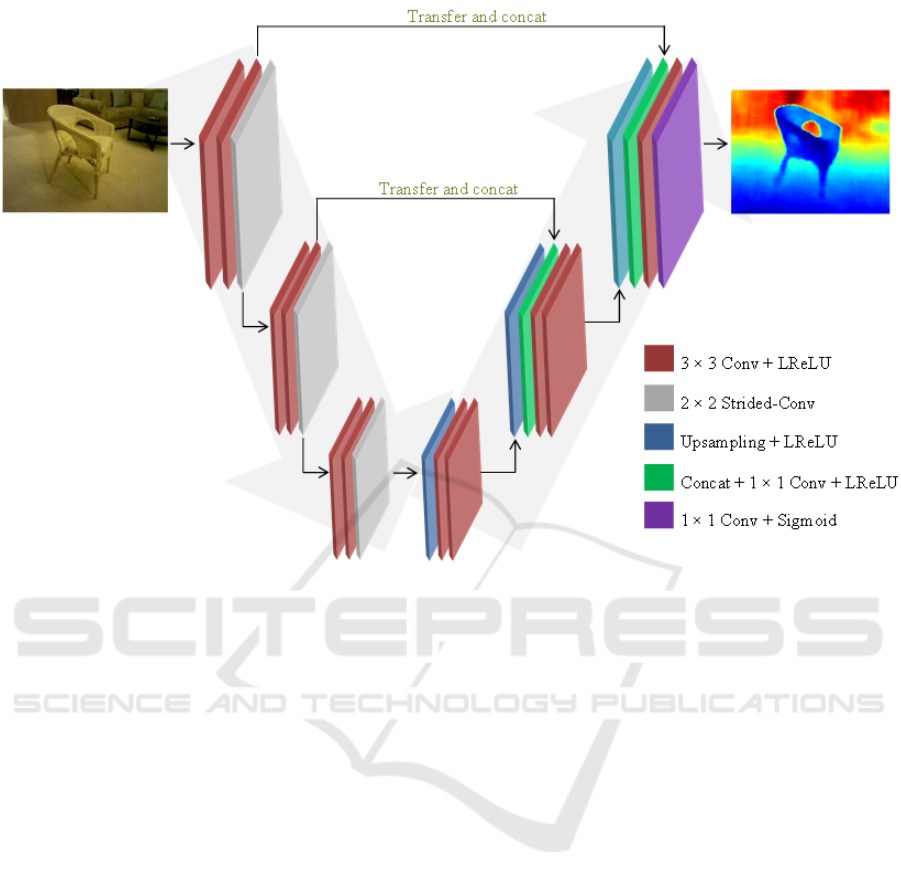
Figure 1: The proposed mini strided V-Net architecture. Pooling layers are replaced by strided-convolutional layers to generate

ﬁne-grained output of same resolution as that of the input. Depth images are visualized with log scale.

output of some layers from the encoder part with the

corresponding output of the upsampling layers from

the decoder part as shown in Fig. 1 (the concatenation

links between the encoder part and the decoder part).

After the concatenation, we apply a convolutional op-

eration of 1 × 1 kernel size to fuse the concatenated

feature maps. We noticed that the concatenation lay-

ers (or as they are called the skip connections) add

more details, and as a consequence, the objects in the

output images have sharper edges and hence are less

blurry. The depth image is generated using a sigmoid

layer as the output range is between the interval of

(0,1).

Generally speaking, the encoder-decoder models

have been introduced into many computer vision tasks

such as semantic segmentation, image reconstruc-

tion, and optical ﬂow estimation. They have signiﬁ-

cantly outperformed other models in solving the same

tasks. The encoder-decoder models have shown im-

pressive success in solving single-view depth estima-

tion for scenes in supervised and unsupervised train-

ing modes. In the results section, we will compare the

proposed model with other models and show that the

proposed encoder-decoder model outperforms other

models and can generate better depth images with

more details.

3.2 Loss Function

Selecting a suitable loss function plays a critical step

in training a CNN. In our case, the loss function mea-

sures the error between the generated depth image

and the ground-truth depth image to optimize and up-

date the model weights. It should fulﬁll some con-

straints regarding the task and the nature of the train-

ing dataset. Our depth estimation problem is consid-

ered as a regression task and a straightforward loss

function like L2 norm can be used to compute the er-

ror between the estimated values

y and the ground-

truth y (Liu et al., 2017).

For depth estimation, L2 norm is not robust to out-

liers (the large error calculated between the predicted

depth and the ground-truth) (Liu et al., 2017). Opti-

mizing the model using L2 norm biases the training

process towards the outliers because small errors (dif-

ferences between the ground-truth and the predicted

depth values) have little inﬂuence on the CNN weight

modiﬁcations, while the large errors (outliers) incur a

large penalty.

To overcome this issue, we propose to use a non-

convex loss function that is robust in regression tasks

namely, Tukey’s biweight loss function (Eq. 2) (Black

and Rangarajan, 1996). The advantage of using this

loss function is that the small residual values (the dif-

VISAPP 2020 - 15th International Conference on Computer Vision Theory and Applications

208

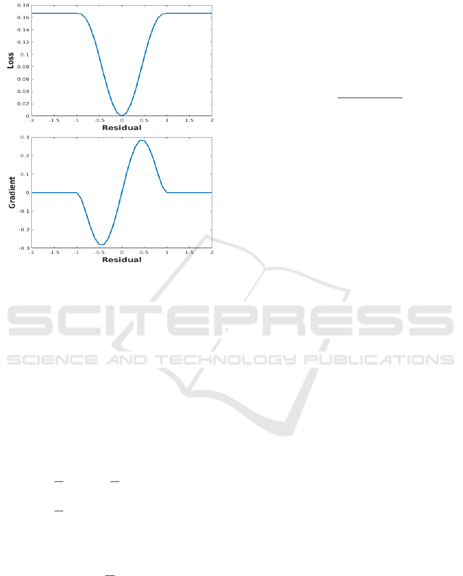
Figure 2: Tukey’s biweight loss function (top) and its ﬁrst-

order derivative (bottom) where c = 1.

ference between the predicted depth and the ground-

truth depth) inﬂuence the training process and robust

to the outliers. During the training process, the loss

function suppresses the inﬂuence of the outliers and

sets the magnitude of the outlier gradients close to

zero.

Formally, the difference between the ground-truth

depth y and the estimated depth value

y (i.e. the resid-

ual r) is calculated as:

r = ˆy − y (1)

Given the residual r (Eq. 1), Tukey’s biweight loss

function is deﬁned by:

ρ(r) =











1 −

if |r| ≤ c

if |r| > c

(2)

The ﬁrst-order derivative of Tukey’s biweight loss

with respect to r is deﬁned as:

ρ(r) =











1 −

if |r| ≤ c

0 if |r| > c

(3)

To correctly apply this loss function, the residual

(r) should be scaled (r should be drawn from distri-

bution with unit variance). Median absolute deviation

(MAD) is selected to measure the variability in the

training data to scale the residuals. MAD is deﬁned

as:

MAD

= median(|r

|) (4)

MAD

scales the residuals to obtain the unit vari-

ance. The scaled residual (r

MAD

) is calculated as:

MAD

− ˆy

1.4826 × MAD

(5)

The scaled r

MAD

in Eq. 5 is used by the loss func-

tion Eq. 2 with c = 4.6851. An advantage of using

Tukey’s biweight function as a loss function is that

it is differentiable and the training process converges

better when the depth values are represented in a log

scale. Fig. 2 shows Tukey’s biweight loss and its ﬁrst

derivative when c = 1.

3.3 Dataset & Implementation Details

We use MatConvNet (Vedaldi and Lenc, 2015), a

MATLAB toolbox implementing CNNs for computer

vision applications, to train and evaluate our proposed

model. The weights of the layers are initialized us-

ing Xavier initialization method (Glorot and Bengio,

2010). The model was trained from scratch using

backpropagation. Stochastic Gradient Descent (SGD)

was used to optimize the network with the follow-

ing settings: the momentum was set to 0.9 and the

weight decay was set to 10

−5

. The learning rate was

initialized to 10

−3

and was divided by 10 when the

validation error didn’t change. The training process

was repeated until the validation accuracy stopped in-

creasing.

The proposed model was trained on real images.

The dataset includes RGB images and their corre-

sponding depth image of real objects. A Large

Dataset of Object Scans (Choi et al., 2016) is a pub-

licly available dataset that contains more than tens of

thousands of 3D scans of different real objects cap-

tured at a resolution of 640×480. We collected dif-

ferent scenes from the chair class. The collected set

was split into a training set and a testing set with a

respective distribution of 80% and 20%, respectively.

The main model was trained using Tukey’s biweight

loss function. We selected the chair object because

the dataset has a massive number of images with di-

versity in shapes. The network was trained on almost

10 different shapes of chairs. Each chair shape was

between 1k and 2k images of different viewpoints and

distances in both indoor and outdoor scenes. We ap-

plied a pre-processing step on the depth images to ﬁll

the missing depth values in the images as shown in

Fig. 3.

Mini V-Net: Depth Estimation from Single Indoor-Outdoor Images using Strided-CNN

209

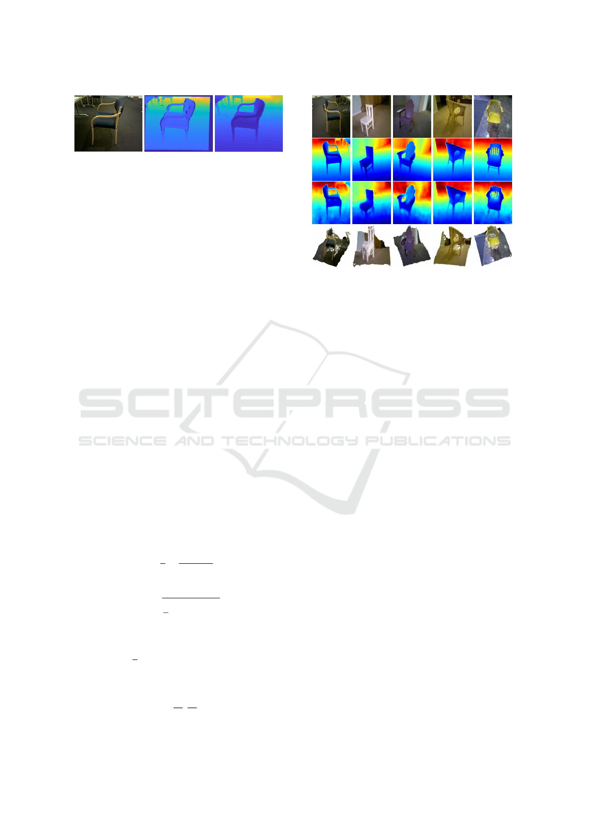
Figure 3: A sample of a training RGB image with a depth

image. From left to right: RGB image, original depth im-

age, and preprocessed depth image.

We applied data augmentation on the training set

to reduce the overﬁtting during training and for bet-

ter generalization performance. Horizontal ﬂipping

(mirroring) of images is applied at a probability of

0.5. Vertical ﬂipping on indoor scene images will not

help during training. Also, we applied photo-metric

transformation, i.e. swapping the color channels of

the RGB images, to increase the performance.

4 EXPERIMENTAL RESULTS

AND DISCUSSIONS

In this section, we report thorough analyses and re-

sults of the proposed model on single-view depth es-

timation in indoor and outdoor scenes. Moreover, we

perform ablation studies to analyze the impact of the

loss functions on the results. Finally, we compare and

discuss the results and the performance of the pro-

posed model to other state-of-the-art models that used

the same dataset for training and testing. The results

(qualitatively and quantitatively) show that the pro-

posed model with non-convex loss function performs

better than the other models and other loss functions

that are used in the regression tasks. For the quan-

titative evaluation and comparison, the same metrics

used in (Aﬁﬁ and Hellwich, 2016) are computed on

our experimental results. The error metrics are de-

ﬁned as:

• Average Absolute Relative Error (rel):

∑

− ˆy

(6)

• Root Mean Square Error (rms):

∑

− ˆy

)

(7)

• Average log

error (log

∑

|log

) − log

( ˆy

)| (8)

• Threshold accuracy (δ

): % of ˆy

s.t.

max(

ˆy

) < δ

(9)

Figure 4: Qualitative results from Large Dataset of Object

Scans (chosen from the testing dataset). From top to bot-

tom: input RGB images, the ground-truth images, the pre-

dicted depth image, and the reconstructed images using the

predicted depth values.

where δ

= 1.25

, i = 1, 2, 3

is a pixel in ground-truth depth image y, ˆy

is a

pixel in the predicted depth image ˆy, and n is the total

number of pixels for each depth image.

4.1 Mini V-Net Evaluation on Large

Dataset of Object Scans

Fig. 4 shows the depth estimation results that are

predicted using the proposed model. The predicted

depth images have the object details and can be eas-

ily distinguished from the background. The ﬁne de-

tails of the objects such as the holes in the back of the

chairs are predicted accurately and the network suc-

ceeds to estimate the objects’ parts. Interestingly, the

proposed model predicts depth information directly

from a single input image without any further post-

processing steps. The model is trained end-to-end to

estimate the depth of an image in a single shot. On

the other hand, other previously described methods

improved the predicted depth images through many

steps. One method (Eigen and Fergus, 2015) uses

a multi-stage model and combines the coarse depth

image generated in one stage and the original RGB

input image to generate the ﬁnal depth image. This

may introduce noise and reduce global scale depth

information. Of note, the output resolution usually

is smaller than the input resolution and many details

may be missed. Moreover, CRF is used as a post-

processing step to generate a more detailed depth im-

age (Liu et al., 2015). As a result, the predicted depth

image cannot be estimated directly from the CNN.

However, our model differs from these models in be-

VISAPP 2020 - 15th International Conference on Computer Vision Theory and Applications

210

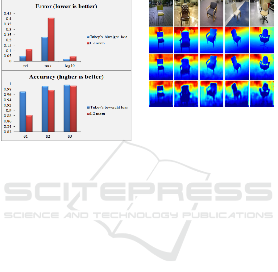
Figure 5: Error (top) and Accuracy (bottom) results of the

proposed model using different loss functions.

ing a single stage model whereby no post-processing

steps are required to generate the output.

Moreover, we reconstruct the images in 3D using

the predicted depth values as shown in Fig. 4 (the

last row). It clearly is shown that the depth values

were predicted very well and there are different levels

of depth values that can distinguish between object

parts, the ﬂoor, and the background.

4.2 Analysis of Different Loss Functions

We trained the proposed model using two different

loss functions; L2 norm and Tukey’s biweight loss.

In our task, the small difference between the depth

values is important because these values highlight the

basic features of the object and differentiate it from

other objects in the scene. We compared the error

and the accuracy of the estimated depth from Tukey’s

biweight loss with the one from L2 norm loss quan-

titatively. Fig. 5 (top) shows that the error com-

puted from Tukey’s biweight loss model is smaller

than the model trained on L2 norm with a large mar-

gin. Also, the accuracy (bottom) when using the non-

convex loss function is better for training the model

in the regression problems.

Fig. 6 elucidates that the model trained using

Tukey’s biweight loss outperforms the model trained

using L2 norm. In detail, the pixels with smaller dis-

tances are sensitive to smaller errors. This inﬂuences

the relative error to be higher and results in larger gra-

dients of Tukey’s biweight loss over L2 norm. Conse-

Figure 6: Qualitative comparison results on Large Dataset

of Object Scans using different loss functions. From top

to bottom: input RGB image, ground-truth, model trained

using Tukey’s biweight loss, model trained using L2 norm.

Depths are shown in log scale and in color (blue is close,

red is far).

quently, the non-convex loss function is more robust

to the outliers and takes care of the small errors be-

tween distances such that the output is estimated with

ﬁner details compared to L2 norm model. Fig. 6 also

shows that the results predicted by the model trained

using L2 norm are relatively blurry depth images and

the object details are almost missed (the forth row in

Fig. 6). Some object parts are fused with the back-

ground and the object details are not visible. On the

other hand, the depth images generated by Tukey’s bi-

weight loss have captured ﬁner details and the object

inside the images can be recognized easily from the

background. In addition, the network learns to pre-

serve some details related to object shapes such as the

holes in the chair’s hands and the empty space be-

tween the back of the chair and seat.

4.3 Comparison with Other Models

Depth estimation from a single image is an ambigu-

ous task. We compare the proposed model with (Aﬁﬁ

and Hellwich, 2016) which used the same dataset for

training but their model is different. Their CNN is a

fully convolutional model that simply used convolu-

tional layers and pooling layers and the output was

generated from a sigmoid function. Moreover, they

trained the fully-CNN with Tukey’s biweight loss

similar to our approach. Table 1 shows the quanti-

tative comparison with respect to errors and accuracy.

Fig. 7 shows the qualitative results predicted by our

model along with a comparison to those generated by

the model in (Aﬁﬁ and Hellwich, 2016).

The model in (Aﬁﬁ and Hellwich, 2016) was

Mini V-Net: Depth Estimation from Single Indoor-Outdoor Images using Strided-CNN

211

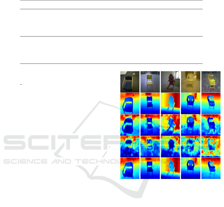
Table 1: Performance Comparison of different methods trained using different loss functions on Large Dataset of Object

Scans (↓ lower is better, ↑ higher is better).

Architecture rel↓ rms↓ log10↓ δ

↑ δ

↑

Models trained using Tukey’s biweight loss

F-CNN (full) (Aﬁﬁ and Hellwich, 2016) 0.2940 0.9516 0.1264 0.4895 0.7958 0.9205

F-CNN (half) (Aﬁﬁ and Hellwich, 2016) 0.2341 0.7644 0.0970 0.5971 0.8940 0.9720

Ours 0.0507 0.2314 0.0218 0.9713 0.9927 0.9972

Models trained using L2 norm

F-CNN (full) (Aﬁﬁ and Hellwich, 2016) 0.3047 1.2146 0.1661 0.3771 0.6662 0.8344

F-CNN (half) (Aﬁﬁ and Hellwich, 2016) 0.2571 0.9976 0.1317 0.4453 0.7794 0.9202

Ours 0.1150 0.4104 0.0479 0.8825 0.9772 0.9935

trained on different image resolutions. For each reso-

lution, the network generated the depth image that had

a size of

of the input image size. This is because

the model uses two pooling layers which decreases

the image resolution twice. Pooling layers are used

to decrease the computational costs and reduce the

feature dimensions. However, some features are lost

from these layers. Our proposed model is an encoder-

decoder model where deconvolutional layers (upcon-

volutional layers) are used to reconstruct the image

again to its original resolution. Using these layers al-

lows us to solve the issues related to the output resolu-

tion. Furthermore, we use skip connections between

the encoder and the decoder. The purpose of the skip

connections is to transfer useful information that has

been extracted from the encoder part and utilize them

when predicting the depth information in the decoder

part. These connections improve the quality of the

generated images and make the objects’ parts sharper.

The object parts and the holes in the chairs can be

easily recognized from the depth images generated by

our encoder-decoder model. To decrease the feature

dimensions, we use strided convolutional layers that

have features to be learned and can extract useful fea-

tures, unlike the pooling layers. Also, they preserve

the spatial location of the information and feed them

to the next layer during the training.

As shown in Fig. 7, the predicted depth images

using the proposed method is better than the ones pre-

dicted using (Aﬁﬁ and Hellwich, 2016) that they con-

tain more details. Moreover, our method predicts the

depth at a higher quality where the edges and the holes

almost match the ground-truth images with fewer ar-

tifacts.

5 CONCLUSION

Single-view depth estimation is an extremely chal-

lenging problem. In this paper, we proposed a

Figure 7: Qualitative comparison results on Large Dataset

of Object Scans. From top to bottom: input image, ground-

truth, F-CNN (Aﬁﬁ and Hellwich, 2016) trained on Tukey’s

biweight loss, F-CNN (Aﬁﬁ and Hellwich, 2016) trained on

L2 norm, and ours. Depths are shown in log scale and in

color (blue is close, red is far).

light and simple fully-convolutional encoder-decoder

model for depth estimation from a single RGB im-

age. Unlike the traditional models that require multi-

stage or post-processing steps to predict the depth,

our model is a simple single-stage model that predicts

the depth images directly without any further post-

processing steps. By contrast to other methods, that

struggle to generate high-resolution images, the gen-

erated depth images using the proposed model have

the same resolution as that of the input images. We

demonstrate that the loss function inﬂuences the ﬁnal

output, and for our speciﬁc problem the non-convex

loss functions are more suitable for regression tasks

because they are robust to the outliers. We show

VISAPP 2020 - 15th International Conference on Computer Vision Theory and Applications

212

that our simple and well-designed model outperforms

other models on the same datasets and using the same

loss functions during training. Our work generates

high-quality depth images that capture the boundaries

and reveal ﬁner parts such as the holes in the back.

We believe that the encoder-decoder model for

depth estimation can be applied within areas such as

scene depth estimation of monocular SLAM and the

depth information can be utilized for further applica-

tions such as semantic segmentation and scene recon-

struction.

REFERENCES

Aﬁﬁ, A. J. and Hellwich, O. (2016). Object depth esti-

mation from a single image using fully convolutional

neural network. In 2016 International Conference on

Digital Image Computing: Techniques and Applica-

tions (DICTA), pages 1–7. IEEE.

Black, M. J. and Rangarajan, A. (1996). On the uniﬁcation

of line processes, outlier rejection, and robust statis-

tics with applications in early vision. International

Journal of Computer Vision, 19(1):57–91.

Cao, Y., Wu, Z., and Shen, C. (2018). Estimating depth

from monocular images as classiﬁcation using deep

fully convolutional residual networks. IEEE Transac-

tions on Circuits and Systems for Video Technology,

28(11):3174–3182.

Choi, S., Zhou, Q.-Y., Miller, S., and Koltun, V. (2016).

A large dataset of object scans. arXiv preprint

arXiv:1602.02481.

Dalal, N. and Triggs, B. (2005). Histograms of oriented

gradients for human detection. In international Con-

ference on computer vision & Pattern Recognition

(CVPR’05), volume 1, pages 886–893. IEEE Com-

puter Society.

Eigen, D. and Fergus, R. (2015). Predicting depth, surface

normals and semantic labels with a common multi-

scale convolutional architecture. In Proceedings of

the IEEE international conference on computer vi-

sion, pages 2650–2658.

Eigen, D., Puhrsch, C., and Fergus, R. (2014). Depth map

prediction from a single image using a multi-scale

deep network. In Advances in neural information pro-

cessing systems, pages 2366–2374.

Glorot, X. and Bengio, Y. (2010). Understanding the difﬁ-

culty of training deep feedforward neural networks.

In Proceedings of the thirteenth international con-

ference on artiﬁcial intelligence and statistics, pages

249–256.

Hadsell, R., Sermanet, P., Ben, J., Erkan, A., Scofﬁer, M.,

Kavukcuoglu, K., Muller, U., and LeCun, Y. (2009).

Learning long-range vision for autonomous off-road

driving. Journal of Field Robotics, 26(2):120–144.

He, K., Zhang, X., Ren, S., and Sun, J. (2016). Deep resid-

ual learning for image recognition. In Proceedings of

the IEEE conference on computer vision and pattern

recognition, pages 770–778.

Hoiem, D., Efros, A. A., and Hebert, M. (2005). Automatic

photo pop-up. ACM transactions on graphics (TOG),

24(3):577–584.

Krizhevsky, A., Sutskever, I., and Hinton, G. E. (2012). Im-

agenet classiﬁcation with deep convolutional neural

networks. In Advances in neural information process-

ing systems, pages 1097–1105.

Ladicky, L., Shi, J., and Pollefeys, M. (2014). Pulling things

out of perspective. In Proceedings of the IEEE con-

ference on computer vision and pattern recognition,

pages 89–96.

Liu, B., Gould, S., and Koller, D. (2010). Single image

depth estimation from predicted semantic labels. In

2010 IEEE Computer Society Conference on Com-

puter Vision and Pattern Recognition, pages 1253–

1260. IEEE.

Liu, F., Lin, G., and Shen, C. (2017). Discriminative train-

ing of deep fully connected continuous crfs with task-

speciﬁc loss. IEEE Transactions on Image Processing,

26(5):2127–2136.

Liu, F., Shen, C., and Lin, G. (2015). Deep convolutional

neural ﬁelds for depth estimation from a single image.

In Proceedings of the IEEE Conference on Computer

Vision and Pattern Recognition, pages 5162–5170.

Liu, M., Salzmann, M., and He, X. (2014). Discrete-

continuous depth estimation from a single image. In

Proceedings of the IEEE Conference on Computer Vi-

sion and Pattern Recognition, pages 716–723.

Lowe, D. G. (2004). Distinctive image features from scale-

invariant keypoints. International journal of computer

vision, 60(2):91–110.

Milletari, F., Navab, N., and Ahmadi, S.-A. (2016). V-

net: Fully convolutional neural networks for volumet-

ric medical image segmentation. In 2016 Fourth Inter-

national Conference on 3D Vision (3DV), pages 565–

571. IEEE.

Perronnin, F., S

anchez, J., and Mensink, T. (2010). Im-

proving the ﬁsher kernel for large-scale image classi-

ﬁcation. In European conference on computer vision,

pages 143–156. Springer.

Ren, X., Bo, L., and Fox, D. (2012). Rgb-(d) scene labeling:

Features and algorithms. In 2012 IEEE Conference

on Computer Vision and Pattern Recognition, pages

2759–2766. IEEE.

Roberts, R., Sinha, S. N., Szeliski, R., and Steedly, D.

(2011). Structure from motion for scenes with large

duplicate structures. In CVPR 2011, pages 3137–

3144. IEEE.

Saxena, A., Sun, M., and Ng, A. Y. (2009). Make3d: Learn-

ing 3d scene structure from a single still image. IEEE

transactions on pattern analysis and machine intelli-

gence, 31(5):824–840.

Silberman, N., Hoiem, D., Kohli, P., and Fergus, R. (2012).

Indoor segmentation and support inference from rgbd

images. In European Conference on Computer Vision,

pages 746–760. Springer.

Simonyan, K. and Zisserman, A. (2014). Very deep con-

volutional networks for large-scale image recognition.

arXiv preprint arXiv:1409.1556.

Mini V-Net: Depth Estimation from Single Indoor-Outdoor Images using Strided-CNN

213

Soomro, T. A., Aﬁﬁ, A. J., Gao, J., Hellwich, O., Zheng,

L., and Paul, M. (2019a). Strided fully convolutional

neural network for boosting the sensitivity of retinal

blood vessels segmentation. Expert Systems with Ap-

plications, 134:36–52.

Soomro, T. A., Aﬁﬁ, A. J., Zheng, L., Soomro, S., Gao,

J., Hellwich, O., and Paul, M. (2019b). Deep learn-

ing models for retinal blood vessels segmentation: A

review. IEEE Access, 7:71696–71717.

Springenberg, J. T., Dosovitskiy, A., Brox, T., and Ried-

miller, M. (2014). Striving for simplicity: The all con-

volutional net. arXiv preprint arXiv:1412.6806.

Suwajanakorn, S., Hernandez, C., and Seitz, S. M. (2015).

Depth from focus with your mobile phone. In Pro-

ceedings of the IEEE Conference on Computer Vision

and Pattern Recognition, pages 3497–3506.

Szegedy, C., Liu, W., Jia, Y., Sermanet, P., Reed, S.,

Anguelov, D., Erhan, D., Vanhoucke, V., and Rabi-

novich, A. (2015). Going deeper with convolutions.

In Proceedings of the IEEE conference on computer

vision and pattern recognition, pages 1–9.

Vedaldi, A. and Lenc, K. (2015). Matconvnet: Convolu-

tional neural networks for matlab. In Proceedings of

the 23rd ACM international conference on Multime-

dia, pages 689–692. ACM.

Xu, B., Wang, N., Chen, T., and Li, M. (2015). Empiri-

cal evaluation of rectiﬁed activations in convolutional

network. arXiv preprint arXiv:1505.00853.

Zhang, R., Tsai, P., Cryer, J. E., and Shah, M.

(1999). Shape-fromshading: a survey. pattern anal-

ysis and machine intelligence. IEEE Transactions on,

21(8):690–706.

VISAPP 2020 - 15th International Conference on Computer Vision Theory and Applications

214