
Combining Spatial Data Layers using Fuzzy Inference Systems:
Application to an Agronomic Case Study
Serge Guillaume
1 a
, Terry Bates
2 b
, Jean-Luc Labl
´
ee
1
, Thom Betts
3
and James Taylor
1 c
1
ITAP, Univ Montpellier, INRAE, Montpellier SupAgro, Montpellier, France
2
Cornell Lake Erie Research and Extension Laboratory, Cornell University, New-York, U.S.A.
3
Betts Vineyard LLC, New-York, U.S.A.
Keywords:
Fusion, Multicriteria, Preference, Decision.
Abstract:
This paper presents an application of Fuzzy Logic, well known for its linguistic modeling ability, in a multi-
criteria decision making framework applied to spatial data sets. The Fuzzy Logic is integrated in two different
ways. First, fuzzy sets are used to model an expert preference relation for each of the individual spatial infor-
mation sources to turn raw data into satisfaction degrees. Second, fuzzy rules are used to model the interaction
between sources to aggregate the individual degrees into a global score. The whole framework is implemented
in an open source software called GeoFIS. The potential of the method is illustrated using a typical farm-
ing decision: the design of a nitrogen fertilization map within a vineyard. The vineyard is a Concord (Vitis
labrusca) juice grape vineyard in the Lake Erie region of New York state. The vineyard manager and a lo-
cal research/extension viticulturist both used the tool to generate a prescription nitrogen map based on their
knowledge and spatial crop and soil information. The process captured different preferences between the two
users (industry vs. research) and generated different prescription maps that reflected their differing objectives,
knowledge and risk perception in vine management. Although applied to vineyard data, this decision tool has
a wide potential application to agri-environmental (and other) spatial data sets.
1 INTRODUCTION
Complex systems, such as agricultural production
systems, are characterized by several interrelated di-
mensions, for instance agronomic, social and eco-
nomic. The production process includes different
steps performed systematically, from initial selection
of the product type right the way through to product
marketing. Decisions are made at each step of this
process that may degrade or support the sustainability
of the production system.
Decision making often involves several, poten-
tially conflicting, attributes. Multicriteria decision
analysis (MCDA) has been indicated as an appropri-
ate set of tools. In a recent paper (Cinelli et al., 2014)
five MCDA methods were evaluated for their abil-
ity to handle sustainability problems using ten com-
parison criteria. The methods were from three main
families: i) utility-based theory: Multi-Attribute Util-
a
https://orcid.org/0000-0002-3546-5276
b
https://orcid.org/0000-0002-6719-9435
c
https://orcid.org/0000-0001-9709-8689
ity Theory (MAUT) and Analytical Hierarchy Process
(AHP), ii) outranking relation theory: elimination and
choice expressing the reality (ELECTRE) and pref-
erence ranking organization method for enrichment
of evaluations (PROMETHEE) and, iii) the sets of
decision rules theory: Dominance-based Rough Set
Approach (DRSA). The latter uses crisp “if . . . then”
rules where the satisfaction degree for each criterion
is compared to a defined threshold and the conclusion
is a category or a set of categories.
In this work, a generic methodology, implemented
as an open source software is introduced. The pro-
posed framework first converts raw data into satis-
faction degrees according to the decision to be made
and then aggregates these degrees to compute a global
score. The first step is carried out using fuzzy sets:
they are used to model the expert preference relation
for each individual information source. The second
step usually involves numerical operators of aggrega-
tion, including the well known Weighted Arithmetic
Mean (WAM), as well as the Ordered Weighted Aver-
age (OWA). An introduction to these operators can be
found in (Bloch, 1996; Dujmovi
´
c et al., 2009). Few
62
Guillaume, S., Bates, T., Lablée, J., Betts, T. and Taylor, J.
Combining Spatial Data Layers using Fuzzy Inference Systems: Application to an Agronomic Case Study.
DOI: 10.5220/0009356000620071
In Proceedings of the 6th International Conference on Geographical Information Systems Theory, Applications and Management (GISTAM 2020), pages 62-71
ISBN: 978-989-758-425-1
Copyright
c
2020 by SCITEPRESS – Science and Technology Publications, Lda. All rights reserved
20 25 30
0
1
X
x
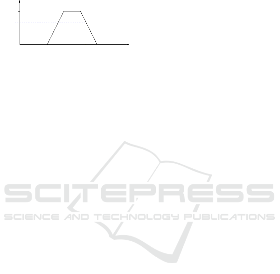
(x)
15
µ
Medium
Figure 1: A Trapezoidal Shaped Fuzzy Set.
papers from the GIS community have utilized these
kind of operators (Shorabeh et al., 2019), and the most
popular technique for multicriteria decision making
remains the AHP (El Jazouli et al., 2019; Seyedmo-
hammadi et al., 2019; Graff et al., 2019; Konstantinos
et al., 2019; Giamalaki and Tsoutsos, 2019).
An alternative to numerical operators is proposed
here to aggregate the satisfaction degrees: a set of
fuzzy rules within a fuzzy inference system. Fuzzy
rules are suitable, and easy to define, to model the in-
teractions between individual variables.
The potential of the method is illustrated using an
agronomic case study: how much nitrogen fertilizer
should be applied according to the production target,
the expert knowledge and the data?
The paper is organized as follows. The basics
of fuzzy logic and linguistic modeling are recalled
in Section 2. The different steps and options of the
multicriteria methodology are introduced in Section
3. Section 4 describes the agronomic case study and
discusses the results. Finally, the main conclusions
are summarized in Section 5.
2 LINGUISTIC MODELING
Fuzzy logic is widely used as an interface between
symbolic and numerical spaces, allowing the imple-
mentation of human reasoning in computers. Fuzzy
sets are used to implement approximate concepts, e.g.
Medium. They are defined using a function that as-
signs to any value, x, in the universe of the variable,
e.g. Temperature, a membership degree, 0 ≤ µ(x) ≤ 1,
as shown in Figure 1. Therefore, in this example,
these degrees would be interpreted as the level to
which x should be considered as a Medium Temper-
ature.
The core of the fuzzy system, Figure 2, is a set of
fuzzy “if . . . then” rules in the form: If Temperature is
Medium then. . . When several variables are involved
in the rule description, the membership degrees can
be combined using an ‘AND’ operator (the most com-
mon are the minimum and the product) to weight
the rule conclusion. The inferred output results from
the aggeregation of all rule conclusions. The rule
base may include expert rules and rules learned from
data, making fuzzy inference systems a suitable en-
vironment for cooperation between expert knowledge
and data mining/learning techniques (Guillaume and
Charnomordic, 2012). As a consequence of overlap
in the fuzzy partition, several rules are likely to be
called by the same input data. The inferred output
is the result of the combination of all these weighted
conclusions.
3 DATA FUSION AND
MULTICRITERIA DECISION
MAKING
The objective here is to ensure that the process of data
fusion for decision making is driven by expert knowl-
edge. Information fusion is done with a specific goal,
for instance risk level evaluation or variable rate ap-
plication in agriculture. The selection of the relevant
and available information sources is done by the de-
cision maker. The next step is to evaluate the possible
level of decision, e.g. risk or rate, according to each of
the sources for a given entity defined by its spatial co-
ordinates. The final step comes down to aggregating
these partial levels, or degrees, to make the final deci-
sion. The aggregation function models the decision-
maker’s preferences: Are some attributes more im-
portant than others? How to combine conflicting in-
formation sources?
The whole framework can be illustrated as fol-
lows:
(a
1
, .. . , a
n
) , (b
1
, . . . , b
n
)
A
−→ f(a) , f(b)
↑ c ↓
(x
1
, . . . , x
n
) , (y
1
, . . . , y
n
) ≺
∼
(a, b)
There are two steps to formalize expert knowledge
and preferences in the decision process. The first
deals with each individual variable, or information
source. The second addresses the interaction between
sources.
The first step aims to turn raw data into satisfac-
tion degrees. This is done by defining a preference
relation for the considered attribute: What are the pre-
ferred values for the decision for this variable? Do
some of these values have a similar meaning for the
decision to be made? Once the values are commen-
surable, i.e. they have the same scale with the same
meaning, they can be aggregated in a second step to
compute a global score. Items can be compared ac-
cording to their score. These two steps are now de-
Combining Spatial Data Layers using Fuzzy Inference Systems: Application to an Agronomic Case Study
63
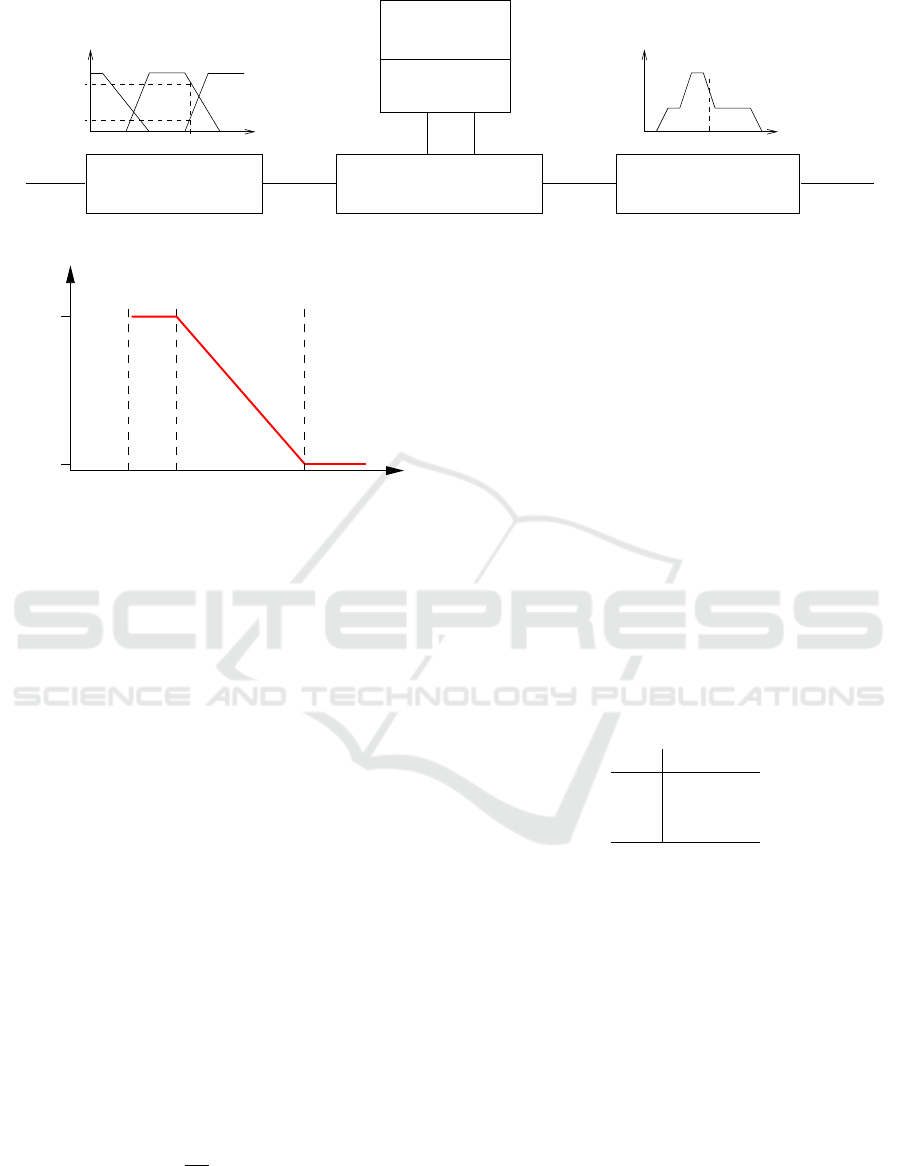
output
output
If...Then
inputinput
base
Fuzzy rule
Defuzzification
crisp fuzzy crisp
Inference engineFuzzification
fuzzy
High
x
µ
(x)
M
(x)
Low Med
H
µ
Figure 2: A Fuzzy Inference System.
0
1
0
i j Pests
Degree
Figure 3: A Membership Function Indicating the Number
of Plant Pests Present and the Corresponding Degree of
Plant Health.
tailed.
3.1 From Raw Data to Satisfaction
Degrees
A common scale with a common meaning is required
by the aggregation process. This step is thus manda-
tory to aggregate information sources with different
scales and different units. It is carried out by asso-
ciating a preference relation to a variable to define
a criterion. The preference depends on the decision
to be made and on the attribute used in the decision-
making. For example, if crop health is evaluated us-
ing the number of plant pests present, then the lower
the number of pests the better the health state. In this
work, the scale is the unit interval, [0, 1] with zero
meaning the criterion is not satisfied and that it is fully
satisfied with one. The preference relation can be
modeled, or implemented, using a fuzzy set as shown
in Figure 3 for this example.
The degrees are computed for any x ∈ [0, +∞[ ac-
cording to Equation 1.
deg(x) =
1 i f x ≤ i
j−x
j−i
i f i ≤ x ≤ j
0 i f x ≥ j
(1)
This is another way of using the fuzzy set concept.
The transformation function includes the part of the
expert knowledge related to each individual variable,
without considering its interaction with the other vari-
ables.
3.2 Numerical Operators
The most popular techniques to aggregate commensu-
rable degrees are numerical operators. The two main
families of such operators, with suitable properties,
are the Weighted Arithmetic Mean (WAM) and Or-
dered Weighted Average (OWA).
The WAM aggregation is recalled in Equation 2.
WAM(a
1
, . . . , a
n
) =
n
∑
i=1
w
i
a
i
(2)
with w
i
∈ [0, 1] and
∑
n
i=1
w
i
= 1. The weights are as-
signed to the sources of information. Unfortunately,
WAM cannot model compromise as shown in this ex-
ample. Let’s consider three items described by two
attributes with the following satisfaction degrees:
a
1
a
2
It 1 0.7 0.7
It 2 0.4 1
It 3 1 0.4
Item 1 is preferred to the other two. This leads to
the two conditions for the weights to fulfill:
• Score(It1) > score(It2) =⇒ w
1
> w
2
• Score(It1) > score(It3) =⇒ w
2
> w
1
These two conditions are contradictory, and there is
no combination (w
1
, w
2
) that can model the decision
maker preference.
The OWA (Yager, 1988) is computed as shown in
Equation 3.
OWA(a
1
, . . . , a
n
) =
n
∑
i=1
w
i
a
(i)
(3)
where (.) is a permutation such as a
(1)
≤ · ·· ≤ a
(n)
.
In this case, the degrees are ordered and the
weights are assigned to the locations in the distribu-
tion, from the minimum to the maximum, whatever
GISTAM 2020 - 6th International Conference on Geographical Information Systems Theory, Applications and Management
64
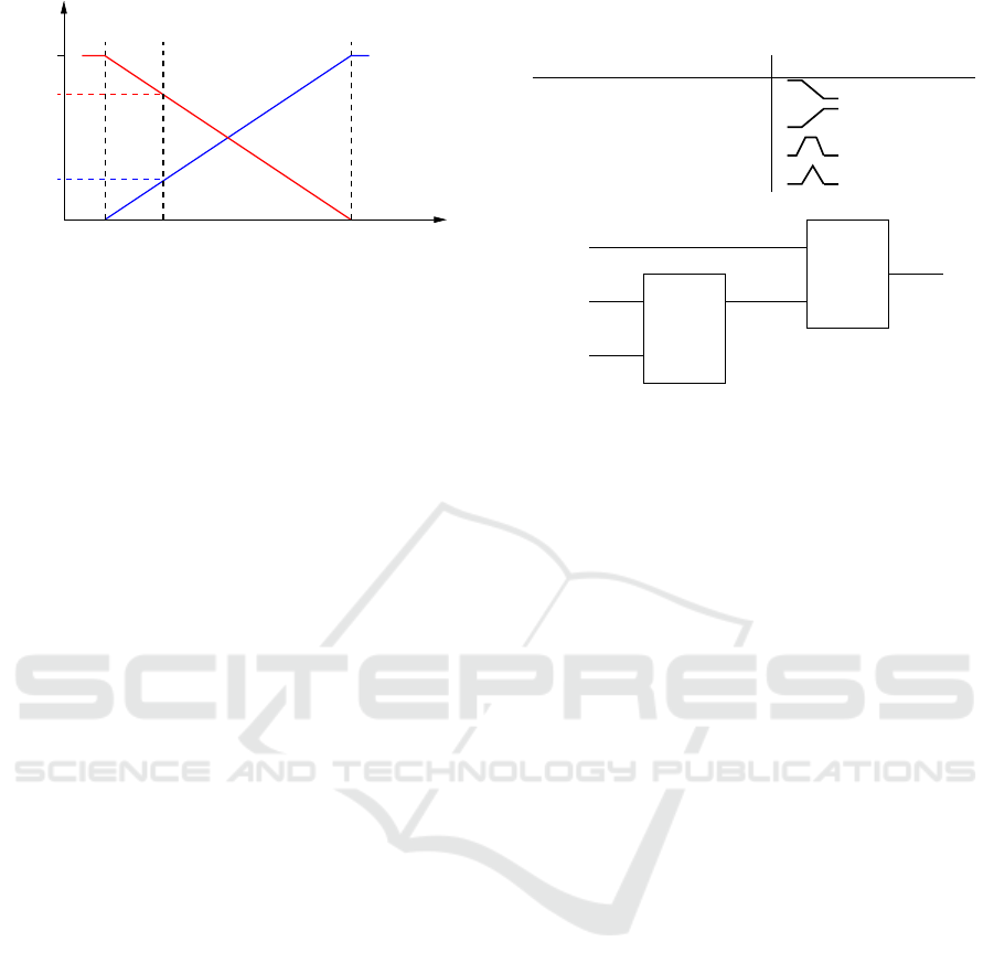
0
1
High
0
Low
0.2
0.2
0.8
Degree1
Figure 4: A Regular Fuzzy Partition with Two Linguistic
Labels.
the information sources. Using the OWA, the two
contradictory conditions above can be solved. WAM
and OWA can be combined in the Weighted OWA op-
erator, WOWA (Torra, 1996).
These operators are easy to use, the number of
parameters is the number of information sources to
aggregate, but their modeling ability is limited. The
Choquet integral (Choquet, 1954) proved to be use-
ful in multi-criteria decision making (Grabisch and
Labreuche, 2008). It is computed according to Equa-
tion 4.
C(a
1
, . . . , a
n
) =
n
∑
i=1
(a
(i)
− a
(i−1)
)w(A
i
) (4)
where (.) is a the permutation previously defined with
a
(0)
= 0 and A
i
= {(i), . . . , (n)}, meaning the set of
sources with a degree a ≥ a
(i)
.
The weights are not only defined for each of the
information sources but for all their possible combi-
nations. Specific configurations include WAM and
OWA modeling. In the general case, the aggrega-
tion of n information sources requires 2
n
coefficients.
These are usually set by learning algorithms (Murillo
et al., 2013).
3.3 Fuzzy Inference Systems
A fuzzy inference system usually requires more pa-
rameters than the former numerical aggregators but,
in this particular case of data fusion, the design can
be simplified as all the input variables are satisfaction
degrees that share the same scale, unit interval, and
the same meaning. Strong fuzzy partitions with reg-
ular grids are used to ensure semantic integrity. The
unique parameter left to the user is the number of lin-
guistic terms for each input variable. In this work it
was set at 2, Low and High, for each variable. The au-
tomatically generated input fuzzy partition is shown
in Figure 4. Thus, any degree 0 < x < 1 partially be-
longs to the two sets with a complementary level.
With two linguistic labels per variable, the num-
ber of rules is 2
n
, i.e. the equivalent number of co-
Table 1: Functions to Turn Raw Data into Satisfaction De-
grees.
Name Shape Preference
Semi Trapezoidal Inferior : low values
Semi Trapezoidal Superior : high values
Trapezoidal : an interval
Triangular : a value
S2
S1
In 2
In 1
In 3
Out 1
Out 2
Figure 5: A Hierarchical Structure to Decision-Making
Where the Scaled Output from the First Decision (S1) Is
an Input for the Second Decision (S2).
efficients required by the Choquet integral. A rule
describes a local context that the domain expert, the
decision maker, is able to understand. In this way, the
rule conclusions are easier to define than the Choquet
integral coefficients.
3.4 Implementation
The fusion module is implemented as an open source
software in the GeoFIS program. The data must be
co-located, i.e. a record includes the spatial coordi-
nates, from a point to a zone, and the corresponding
attributes.
The available functions to turn raw data into de-
grees are summarized in Table 1.
Three aggregation operators are currently avail-
able: WAM, OWA and a fuzzy inference system (FIS)
that can use linguistic rules.
For WAM and OWA the weights can be learned
provided a co-located target is available. Rule con-
clusion can also be learned using the FisPro software
(Guillaume and Charnomordic, 2011).
Rule conclusion can be either a linguistic term,
fuzzy output, or a real value, crisp output. Using a
fuzzy output, it would be necessary to define as many
labels as there are different suitable rule conclusions.
As a crisp conclusion may take any value in the output
range, it allows for more versatility.
The output should also range in the unit interval.
This constraint ensures that the output can feed a fur-
ther step of the process as shown in Figure 5.
In this way, the intermediate systems can be kept
small, making their design and interpretation easier.
The GeoFIS program includes a distance function
based on a fuzzy partition that allows for integrat-
Combining Spatial Data Layers using Fuzzy Inference Systems: Application to an Agronomic Case Study
65

ing expert knowledge into distance calculations (Guil-
laume et al., 2013) as well other functionalities, such
as a zone delineation algorithm (Pedroso et al., 2010).
An illustration of its potential use in Precision Agri-
culture can be found in (Leroux et al., 2018).
4 CASE STUDY
In this section a short case study is presented of the
spatial decision support model. It is not possible to
provide an exhaustive case study within the restric-
tions of a conference paper. It is therefore primarily il-
lustrative in nature but based on a typical farming de-
cision, the application of nitrogen within a vineyard.
The vineyard is a Concord (Vitis labrusca) juice grape
vineyard in the Lake Erie region of New York state.
The decision process followed by both a grower and
an academic are presented to illustrate how the dif-
ferent knowledge bases and risk perceptions are cap-
tured in the process. For this illustration, only the FIS
approach is considered and the OWA and WAM op-
erators are not used. Although a relatively simple ex-
ample, the following case study utilizes three differ-
ent types membership functions to derive satisfaction
degrees (both inferior and superior semi-trapezoidal
functions and a trapezoidal function, Table 1). The
degrees are aggregated using a fuzzy rule base.
4.1 The Decision
How much nitrogen fertilizer should be applied to the
vineyard and should this be site-specific?
The amount of fertilizer applied will be dependent
on the intended vine size management and the pro-
duction target, which is likely to differ between grow-
ers. In general terms, larger vines should be more pro-
ductive and ripen more grapes. Management, includ-
ing nutrition, should aim to enable crop maturity and
to maintain vine size. Smaller vines risk being over-
stressed with a large fruit load and will have lower
long-term productivity. They are also more suscep-
tible to cold and disease damage. The intent with
smaller vines is to manage the fruit load and nutrition
so that the vine can put more effort into vegetative de-
velopment in the short-term to increase its size and so
become more productive in the longer-term.
Information was available on soil variability in the
form of an apparent soil electrical conductivity (EC
a
)
map that is a surrogate for soil texture and to some
extent soil fertility. Crop information was available
as vine size (measured as pruning mass) and Crop
Load (the ratio of the mass of fruit to pruning mass).
These data were obtained from various sensors (see
Table 2: Membership Functions Defined by a and B to
Standardize the Input Variables into a [0, 1] Range and to
Identify What Constitutes a Good (1) and Bad (0) Score.
The Soil EC
a
Variable Was Defined Jointly by the Two
Decision-Makers and Is Constant. The Pruning Mass and
Crop Load Were Defined Independently and Illustrate a Dif-
ference in Opinion between the Two on What Is the Mini-
mum Value for a Good Vine Size and a Bad Crop Load.
Soil conductivity Pruning Mass CropLoad
EC
a
(mS/m) (lbs/vine) (Ravaz Index)
A
1 - 2 10 - 18
B
2, 10, 15, 33 1 - 2.5 10 - 15
(Bates et al., 2018) for further details) and mapped
onto a common grid. The interpolated data are shown
in Figure 6 to illustrate general (and differing) trends
between the variables.
Within this case study, the thought process of two
decision-makers was used to illustrate the flexibility
in the decision systems and the potential to arrive at
different outcomes from identical inputs based on the
specific objectives of each individual decision-maker.
The first decision-maker, denoted “A”, is the vineyard
owner/manager, who routinely makes decisions in the
vineyard to ensure the viability of the production sys-
tem. Their decision-making is strongly influenced by
the accumulated knowledge of 3 generations of vine-
yard management in the region.
The second decision-maker is a trained viticultur-
ist, denoted “B”, who is involved in research and ex-
tension activities in the district. B is also a vineyard
manager, but their knowledge is strongly informed
from the scientific literature, rather than a family his-
tory in vineyards.
4.2 The Aggregation System
The first step is to allow each decision-maker to im-
pose their knowledge onto the input variables. The
decision is based on managing larger and smaller
vines; but what is a large and small vine? Similarly,
what soil EC
a
response is considered good or bad
from a nutritional perspective? To define this, mem-
bership functions were generated (Table 2) to transfer
the decision-makers preferences into the analysis and
also to standardized inputs to a [0,1] range for future
analysis.
There was agreement between A and B on the E C
a
function so it is common for both decision paths. Note
that in the EC
a
layer, very low and very high values
are both considered poor for production, and this is
permissible in the analysis. The two decision-makers
GISTAM 2020 - 6th International Conference on Geographical Information Systems Theory, Applications and Management
66
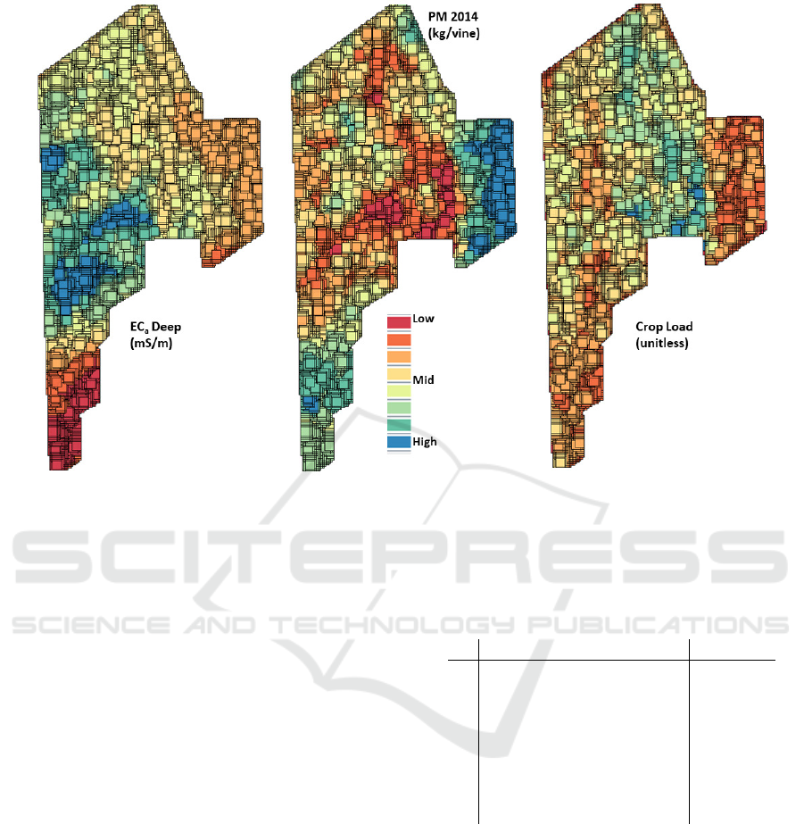
Figure 6: Images Illustrating the Spatial Patterns of the Three Input Variables - Apparent Soil Electrical Conductivity (Left,
EC
a
) to a Depth of 1.5 M Using a Dualem 1s (DUALEM, Mississauga, ON, Canada); Pruning Mass (Centre, PM 2014)
from 2014 Predicted from a Calibrated Canopy Sensor ((Taylor et al., 2017) and Crop Load (Ravaz Index) in 2014 Using the
Pruning Mass and Grape Yield Monitoring Data (Yield Data Not Shown).
differed in their interpretation of good vine size (prun-
ing mass) and desired Crop Load. The vineyard man-
ager (A) considered 2 lbs (0.91 kg) vines as a good
vine size, while the researcher (B) defined 2.5 lbs
(1.13 kg) as the minimum for a good vine size. Simi-
larly, A did not consider the vines over-cropped until
a higher Crop Load value was achieved, i.e. A, the
commercial grower, was more content to have more
fruit in the vineyard, effectively pushing the vines
harder than B through this step. This may stem from
a better understanding of what the vineyard can pro-
duce and/or a need to ensure sufficient short-term pro-
duction to remain economically viable.
Following the specification of the membership
functions, a fuzzy inference system can be used to
define the decisions for A and B. For the three in-
puts, 2 levels of operation [High/Low] were defined.
This gave 8 potential linguistic rules (Table 3). Again,
these rules were defined jointly by A and B in agree-
ment with the relative amount of nitrogen fertilizer
needed in each situation. Of course, this may not al-
ways be the case, and producers with differing objec-
tives could generate different “if-then” statements at
this point. However, in this case, the rules were com-
mon for both A and B to simplify the example. Crisp
numerical values were used for the rule conclusions,
Table 3: The Linguistic Rule Base. Abbreviations Refer to
the Variables Presented in Figure 6.
CropLoad EC
a
PM Nitrogen
1 Low low Low 0.7
2 Low low High 0.5
3 Low High Low 0.5
4 Low High High 0.3
5 High low Low 0.9
6 High low High 0.7
7 High High Low 0.7
8 High High High 0.5
such that Line one (Table 3) reads If CropLoad is Low
AND EC
Deep
is Low AND PM is Low then Nitrogen
is 0.7 (i.e. 70% application). As indicated previously,
linguistic or fuzzy outputs could also be possibly used
here for the rule conclusions.
4.3 Results and Discussion
The raw output maps are noisy and difficult to directly
interpret (inset of Figure 7). Of course a variable rate
controller may not have difficult in reading and inter-
preting these maps, although the potential levels of
Combining Spatial Data Layers using Fuzzy Inference Systems: Application to an Agronomic Case Study
67

application may need to be simplified to account for
the application resolution of the variable rate equip-
ment.
For human intervention, and often for simplic-
ity of application, the data can be aggregated into
zones. In this case they are specific nitrogen appli-
cation zones. Figure 7 shows the simplified output for
the decision process of A and B on a common legend.
Note that the legend has yet to be transformed into
actual N values and shows the output (between 0 and
1) from the FIS. The zoning algorithm was performed
using a segmentation approach (Pedroso et al., 2010)
in GeoFIS (Leroux et al., 2018).
In Figure 7 the different satisfaction degrees for
vine size and Crop Load for the two decision makers
have clearly generated some differences in the poten-
tial nitrogen application zones. The inputs were com-
mon, as was the rule set used, so it is not surprising to
see that the pattern of N required is similar in the two
maps. However, seemingly small alterations to the
the idea of a good vine size or an overcropped vine
has clearly affected the final zoning. It is not possible
to say which of the maps is preferable, as each was
tailored to the preferences of each decision-maker.
It is important to note that since the output is stan-
dardized, there does exist another potential point of
difference between A and B in their determination of
how much nitrogen equates to a value of 1 and 0 (and
all values in between) in this situation, or rather, how
much N would each user apply in the red zone, the
yellow zone etc. . . There is no need for this amount to
be fixed for a particular output score.
As indicated in Section 3.4, the rule conclusions
can be specified as a linguistic term (as well as a nu-
merical value. Figure 7 was derived from the numer-
ical rule conclusions in Table 3. However, many pro-
ducers may be more comfortable providing ‘fuzzy’
indications of rates, rather than hard numerical val-
ues. To quickly illustrate this alternative approach,
Table 4 shows the same “if-then” statements as Table
3, but with linguistic rule conclusions. In this case,
the rule conclusions have been specified simply as ei-
ther a ‘High’, ‘Average’ or ‘Low rate’. The decision
process was then rerun, using the same input layers
and the same satisfaction degrees (membership func-
tions) as before, but with the linguistic rule conclu-
sions (Table 4). These were again common for both
A and B. The zoned outcome, for both A and B, is
shown in Figure 8. The output has been defuzzified
and expressed in numerical form ([0,1]).
The two maps in Figure 8 can be compared to each
other (illustrating again the difference in the determi-
nation of satisfaction degrees for Crop Load and vine
size between A and B), or compared to Figure 7. The
Table 4: The Linguistic Rule Base with ’fuzzy’ Linguistic
Rule Conclusions.
CropLoad EC
a
PM Nitrogen
1 Low Low Low High
2 Low Low High Average
3 Low High Low Average
4 Low High High Low
5 High Low Low High
6 High Low High High
7 High High Low High
8 High High High Average
difference between Figures 7 and 8 lies in the use of
the numerical or linguistic rule conclusions (Tables 3
and 4 respectively). The patterns again remain simi-
lar, i.e. areas of higher and lower N application, al-
though the size and shape of the zones, and the loca-
tion of boundaries, is changed. The simpler (3-level)
linguistic rule conclusions have generated smoother
zones than the numerical rule conclusions (with 4 lev-
els). Again, there is no perfect answer here. All four
maps present a solution based on slightly differing in-
put knowledge related to the satisfaction degrees or
the FIS rules. The red zone in the eastern part would
receive the same amount of Nitrogen after the output
maps were translated to actual Nitrogen rates.
This case study has shown the steps involved in a
fertilizer decision process using the data-fusion mod-
ule in GeoFIS and the fuzzy logic option. It illustrates
how even a slight change in the process between users
A and B (with only 2 of the 3 membership functions
varying), generated different prescription levels of N
to be spatially applied in the vineyard. Altering the if-
then rules, and possibly also the types of input infor-
mation preferred by different users for the same deci-
sion, will generate even more pronounced differences.
It is impossible to identify which solution is best, or
if there is an actual optimal solution, as for each case
the outcome is adapted to the perception, risk and ob-
jectives of the user. While the example here is with
fertilizer application, the decision process can be ap-
plied to any decision, provided relevant input layers
and expert knowledge is available.
Finally, it is important to note that although the
software and decision support tool is capable of us-
ing OWA and WAM operators for aggregation, the
agronomic decision selected here (nitrogen applica-
tion) dictated the use of the FIS approach in this in-
stance. The OWA and WAM approaches require well-
structured and logical decision processes i.e. an ag-
gregation of ‘low’ satisfaction degrees should gener-
ate a ‘low’ output response. Agronomic decisions are
not always so linear or straight-forward. In this case,
both small and large vines could receive high applica-
GISTAM 2020 - 6th International Conference on Geographical Information Systems Theory, Applications and Management
68
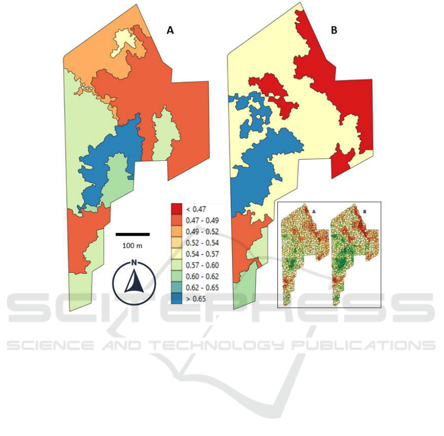
Figure 7: Simplified Zoned Maps (9 Zones Each) of the Nitrogen Decision Generated by the Two Decision-Makers – a =
Vineyard Manager and B = Research Viticulturist. The Raw Output Is Shown in the Inset Image. The Trends Are Similar for
Both, but Boundaries and Output Levels Do Differ.
tions of nitrogen, for differing reasons (see lines 1 and
6 in Tables 3 and 4). For smaller vines, additional ni-
trogen may be needed to promote vegetative vigor to
grow larger, more sustainable vines, while with larger
vines, additional nitrogen will be needed to maintain
a higher level of production under poorer soil condi-
tions. Therefore, the system has two very different
reasons to arrive at the same nitrogen application rate
decision. This is a limitation for the OWA and WAM
operators and a strength for the FIS approach.
5 CONCLUSIONS
This paper has introduced a novel spatial decision
process and demonstrated it using a typical agronomic
practice. The decision process used satisfaction de-
grees specified by the user to avoid the requirement
for a large number of parameters to define input par-
titions and the inference operators. Since all the input
variables in the decision process were satisfaction de-
grees, with a common scale and common meaning,
the automatic setting of the decision rules was possi-
ble using a strong fuzzy partition with linguistic terms
(in this case, Low and High). As a consequence, only
the rule conclusions had to be specifically defined by
the user. This was a relatively quick and easy activ-
ity, using both numerical and linguistic rule conclu-
sions, to allow the expert knowledge (grower, advi-
sor, etc. . . ) of the variables and their interactions to
be modeled. Fuzzy inference systems, thanks to their
proximity with natural language and expert reasoning,
are a good alternative framework for modeling pref-
erences and for use in multi-criteria decision making
under uncertainty.
Field cropping systems operate under a large
amount of uncertainty and variability imposed by
variable biotic and abiotic stresses and a grower’s risk
and market preferences. As such, no decision is ab-
solute. This simple case study illustrated that a dif-
ference in perception of good and bad vine size and
Crop Load (fruit:leaf ratio) generated a difference in
target nitrogen application. The particular novelty of
this decision system was in its ability to provide a
spatial decision that captured the user’s intentions and
Combining Spatial Data Layers using Fuzzy Inference Systems: Application to an Agronomic Case Study
69
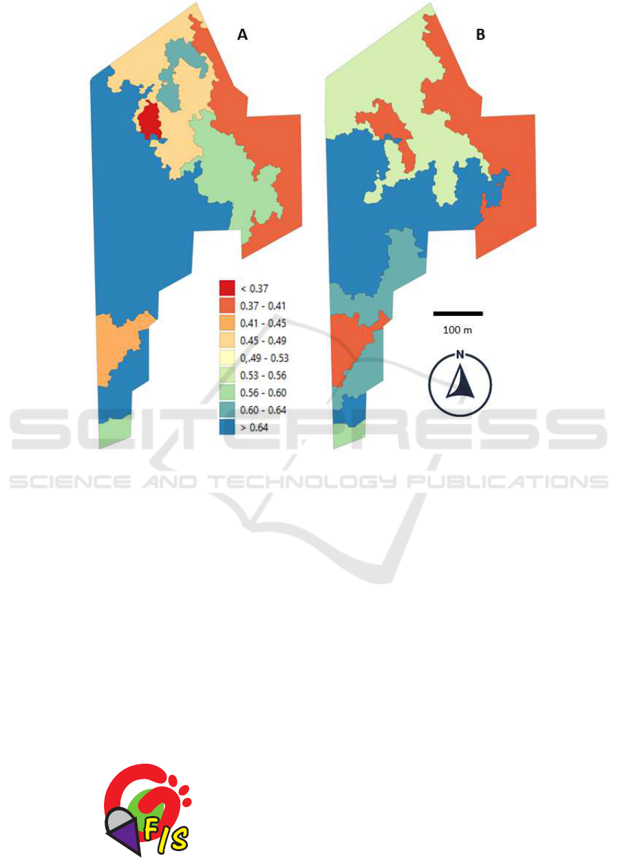
Figure 8: Alternative Nitrogen Application Zones (9 Zones Each) Derived using the Same Satisfaction Degrees and Inputs as
Figure 7, but with Linguistic Rule Conclusions. It Again Shows the Output for Both Users a and B, Illustrating Differences
between Their Choice of Satisfaction Degrees (Table 2). the Use of ‘less Crisp’ Linguistic Rule Conclusions (and Fewer
Levels) Generates More Regular and Larger Zones Compared with the Equivalent Nitrogen Zone Maps in Figure 7.
knowledge without needing the user to understand all
the local, varying interactions in the multi-variate spa-
tial data. The system modeled and spatially differen-
tiated what a grower would do vs. what an advisor
would recommend.
Under these conditions, aggregation with the
OWA and WAM operators was not possible. This is
a limitation for the OWA and WAM operators and a
strength for the FIS approach.
This framework is implemented as an open source
software called GeoFIS available at: https://www.
geofis.org. This is a strong asset as software support
availability is a key factor for a method to be adopted.
ACKNOWLEDGEMENTS
The work is funded by the USDA-NIFA Specialty
Crop Research Initiative Award No. 2015-51181-
24393.
REFERENCES
Bates, T., Dresser, J., Eckstrom, R., Badr, G., Betts, T., and
Taylor, J. (2018). Variable-rate mechanical crop ad-
justment for crop load balance in ‘concord’ vineyards.
In 2018 IoT Vertical and Topical Summit on Agricul-
ture - Tuscany (IOT Tuscany), pages 1–4.
Bloch, I. (1996). Information combination operators for
data fusion: a comparative review with classification.
IEEE Transactions on Systems, Man, and Cybernetics
- Part A: Systems and Humans, 26(1):52–67.
Choquet, G. (1954). Theory of capacities. Annales de
l’Institut Fourier, 5:131–295.
GISTAM 2020 - 6th International Conference on Geographical Information Systems Theory, Applications and Management
70

Cinelli, M., Coles, S. R., and Kirwan, K. (2014). Analy-
sis of the potentials of multi criteria decision analysis
methods to conduct sustainability assessment. Eco-
logical Indicators, 46:138 – 148.
Dujmovi
´
c, J., De Tr
´
e, G., and Dragi
´
cevi
´
c, S. (2009). Com-
parison of multicriteria methods for land-use suitabil-
ity assessment. pages 1404–1409.
El Jazouli, A., Barakat, A., and Khellouk, R. (2019). Gis-
multicriteria evaluation using ahp for landslide sus-
ceptibility mapping in oum er rbia high basin (mo-
rocco). Geoenvironmental Disasters, 6(1).
Giamalaki, M. and Tsoutsos, T. (2019). Sustainable siting
of solar power installations in mediterranean using a
gis/ahp approach. Renewable Energy, 141:64–75.
Grabisch, M. and Labreuche, C. (2008). A decade of ap-
plication of the choquet and sugeno integrals in multi-
criteria decision aid. 4OR, 6(1):1–44.
Graff, K., Lissak, C., Thiery, Y., Maquaire, O., Costa, S.,
Medjkane, M., and Laignel, B. (2019). Characteriza-
tion of elements at risk in the multirisk coastal context
and at different spatial scales: Multi-database integra-
tion (normandy, france). Applied Geography, 111.
Guillaume, S. and Charnomordic, B. (2011). Learning in-
terpretable fuzzy inference systems with fispro. Infor-
mation Sciences, 181:4409–4427.
Guillaume, S. and Charnomordic, B. (2012). Fuzzy in-
ference systems: an integrated modelling environ-
ment for collaboration between expert knowledge and
data using fispro. Expert Systems with Applications,
39:8744–8755.
Guillaume, S., Charnomordic, B., and Loisel, P. (2013).
Fuzzy partitions: a way to integrate expert knowl-
edge into distance calculations. Information Sciences,
245:76–95.
Konstantinos, I., Georgios, T., and Garyfalos, A. (2019).
A decision support system methodology for selecting
wind farm installation locations using ahp and topsis:
Case study in eastern macedonia and thrace region,
greece. Energy Policy, 132:232–246.
Leroux, C., Jones, H., Pichon, L., Guillaume, S., Lamour,
J., Taylor, J., Naud, O., Crestey, T., Lablee, J.-L., and
Tisseyre, B. (2018). Geofis: An open source, decision-
support tool for precision agriculture data. Agricul-
ture, 8(6):73.
Murillo, J., Guillaume, S., Tapia, E., and Bulacio, P. (2013).
Revised hlms: A useful algorithm for fuzzy measure
identificat ion. Information Fusion, 14(4):532–540.
Pedroso, M., Taylor, J., Tisseyre, B., Charnomordic, B., and
Guillaume, S. (2010). A segmentation algorithm for
the delineation of management zones. Computer and
Electronics in Agriculture, 70(1):199–208.
Seyedmohammadi, J., Sarmadian, F., Jafarzadeh, A., and
McDowell, R. (2019). Development of a model using
matter element, ahp and gis techniques to assess the
suitability of land for agriculture. Geoderma, 352:80–
95.
Shorabeh, S., Firozjaei, M., Nematollahi, O., Firozjaei, H.,
and Jelokhani-Niaraki, M. (2019). A risk-based multi-
criteria spatial decision analysis for solar power plant
site selection in different climates: A case study in
iran. Renewable Energy, 143:958–973.
Taylor, J. A., Link, K., Taft, T., Jakubowski, R., Joy, P., Mar-
tin, M., Hoffman, J. S., Jankowski, J., and Bates, T. R.
(2017). A protocol to map vine size in commercial
single high-wire trellis vineyards using “off-the-shelf”
proximal canopy-sensing systems. Catalyst: Discov-
ery into Practice, 1(2):35–47.
Torra, V. (1996). Weighted owa operators for synthesis of
information. In Proceedings of IEEE 5th International
Fuzzy Systems, volume 2, pages 966–971.
Yager, R. R. (1988). On ordered weighted averaging ag-
gregation operators in multicriteria decisionmaking.
IEEE Transactions on Systems, Man, and Cybernet-
ics, 18(1):183–190.
Combining Spatial Data Layers using Fuzzy Inference Systems: Application to an Agronomic Case Study
71
