Using Reinforcement Learning for Optimization of a Workpiece
Clamping Position in a Machine Tool
Vladimir Samsonov
1
, Chrismarie Enslin
1
, Hans-Georg K
¨
opken
2
, Schirin Baer
2
and Daniel L
¨
utticke
1
1
Institute of Information Management in Mechanical Engineering, RWTH Aachen University, Aachen, Germany
2
Siemens AG, Digital Factory Division, Nuernberg, Germany
Keywords:
Reinforcement Learning, Soft Actor-Critic, Supervised Learning, Industrial Manufacturing, Process Optimi-
sation, Machine Tool Optimisation.
Abstract:
Modern manufacturing is increasingly data-driven. Yet there are a number of applications traditionally per-
formed by humans because of their capabilities to think analytically, learn from previous experience and adapt.
With the appearance of Deep Reinforcement Learning (RL) many of these applications can be partly or com-
pletely automated. In this paper we aim at finding an optimal clamping position for a workpiece (WP) with
the help of deep RL. Traditionally, a human expert chooses a clamping position that leads to an efficient, high
quality machining without axis limit violations or collisions. This decision is hard to automate because of the
variety of WP geometries and possible ways to manufacture them. We investigate whether the use of RL can
aid in finding a near-optimal WP clamping position, even for unseen WPs during training. We develop a use
case representing a simplified problem of clamping position optimisation, formalise it as a Markov Decision
Process (MDP) and conduct a number of RL experiments to demonstrate the applicability of the approach in
terms of training stability and quality of the solutions. First evaluations of the concept demonstrate the capa-
bility of a trained RL agent to find a near-optimal clamping position for an unseen WP with a small number of
iterations required.
1 INTRODUCTION
Computer Numerical Control (CNC) machining is
widely used in the manufacturing industry. To pro-
duce a part of a certain geometry, a CNC program
defining relative movements of the cutting tool to the
workpiece (WP) is created as a first step. Addition-
ally, a clamping position of the WP in the milling ma-
chine space has to be chosen manually, solely based
on the human expert knowledge and experience.
The controller translates the relative toolpath into
real axis moves based on the machine kinematics and
the chosen WP clamping position. Therefore, de-
pending on the choice of the WP clamping position,
the tool movements can be conducted by various ma-
chine axes resulting in different levels of processing
speed, quality, machine wear and energy efficiency.
In this study we investigate whether a deep rein-
forcement learning agent (from here on referred to as
the RL agent) can learn a strategy to find a clamp-
ing position close to the optimum for a given WP.
Furthermore, we investigate whether an RL agent
can not only reproduce learned optimal solutions,
but come up with abstract solution strategies capa-
ble of efficiently generalising to new, previously un-
seen, WPs. The RL agent is expected to learn WP
positioning strategies addressing two tasks simulta-
neously: avoiding axis collisions and finding optimal
clamping positions in terms of axis accelerations and
traveled distances.
2 RELATED WORK
Over years many efficient approaches have been
proposed to tackle optimisation tasks. Random
search (Anderson, 1953) and simulated annealing
(van Laarhoven and Aarts, 1987) are conventional
search methods which attempt to approximate the op-
timal solution for optimisation problems. Due to the
large search space for complex problems, calcula-
tion time and computational efforts are enormous and
506
Samsonov, V., Enslin, C., Köpken, H., Baer, S. and Lütticke, D.
Using Reinforcement Learning for Optimization of a Workpiece Clamping Position in a Machine Tool.
DOI: 10.5220/0009354105060514
In Proceedings of the 22nd International Conference on Enterprise Information Systems (ICEIS 2020) - Volume 1, pages 506-514
ISBN: 978-989-758-423-7
Copyright
c
 2020 by SCITEPRESS – Science and Technology Publications, Lda. All rights reserved

the solutions are rather use-case specific than generic.
Genetic search algorithms (Hajela and Lin, 1992) are
more efficient in finding an approximately optimal so-
lution, but there is still a large amount of engineering
effort needed for every different problem definition.
These methods search for the global optimum for a
certain problem while inserting randomness to try and
circumvent possible local optimums. The further dis-
advantages of these methods, besides computational
efforts, include not considering the current state of
the environment during the search, not ”remember-
ing” previous knowledge gained in the optimisation
process and having to be started from scratch every
time.
We are aiming for a solution that is able to gener-
alise to various problems with the possibility of trans-
ferring existing knowledge to new scenarios. The re-
cent success of RL and its powerful ability to solve
complex tasks by trial and error (Vinyals et al., 2019)
inspired the use of this method for our optimisation
problem. As discussed in detail in (Sutton and Barto,
2018), an RL agent has a defined environment that it
interacts with and receives feedback from. The RL
agent will find itself in a state (S) and performs an
interaction with the environment by choosing a spe-
cific action (a), from a finite set of possible actions.
A feedback signal will be returned in the form of a
reward (R) and a definition of the new state (S
0
) will
be provided. The aim is to learn a function approxi-
mation for the policy that chooses the optimal actions.
Q-values are estimations of the future value that each
action could bring and helps in the decision-making
of which action to choose. The value function is an
estimation of the total possible future values.
In this work we use a novel RL Algorithm referred
to as Soft Actor-Critic (SAC) (Haarnoja et al., 2018).
It is an off-policy algorithm based on an actor-critic
architecture. The main peculiarity of the algorithm is
the use of an entropy term as part of the value function
that intensifies exploration in an efficient way. Com-
paring to other off-policy algorithms, SAC is fairly
robust and stable, thus reducing the effort of its appli-
cation to a certain task considerably.
More and more research focuses on the usage of
RL methods in the manufacturing domain, for exam-
ple to solve robot control (Johannink et al., 2019), for
online optimisation of flexible manufacturing systems
in terms of energetic load management (Bakakeu
et al., 2018) and for online job shop scheduling in
flexible manufacturing systems (Baer et al., 2019). At
the same time RL is proved to be an efficient tool for
solving a number of optimisation problems in other
domains. (Li and Malik, 2016) and (Li and Malik,
2017) demonstrate that RL can be used as an optimi-
sation algorithm for high dimensional stochastic op-
timisation problems. Using an RL agent as an op-
timizer for training shallow neural networks or find-
ing an optimal solution for a given objective function
converges faster and/or reaches better optima compar-
ing to commonly used optimisation approaches. A
number of RL Architectures are proposed to solve
combinatorial optimisation problems in (Nazari et al.,
2018), (Bello et al., 2016) and (Kool et al., 2018).
To conclude RL is widely used across various
manufacturing engineering and other domains and
proves to be a capable tool for addressing various op-
timisation tasks.
3 EXPERIMENTAL SETUP
The whole experimental setup is built around the WP
clamping position optimisation problem, formalised
as a sequential decision making process and covers
the setup for the RL agent training and evaluation.
The ultimate goal is to train and evaluate an RL agent
capable of finding a valid and near-optimal clamping
position for seen, as well as unseen WPs. A valid
clamping position is defined as a position that causes
no axis collisions during the milling process. A near-
optimal clamping position for a given geometry offers
close to minimal energy consumption and machine
wear via minimising axis accelerations and total trav-
eled distances along the machine axes.
3.1 Milling Process Description
All investigations are conducted on the simulation of
a 3-Axis milling process using SinuTrain software.
Within the simulation setup various WP geometries
can be generated with a few examples displayed in
Figure 1. The WP geometry changes by varying the
orientation of the slot to be milled into the WP.
For every simulation run, a clamping position for
the WP needs to be defined within the working space
of the milling machine. With respect to the defined
clamping position, SinuTrain simulates the move-
ments of the machine’s axes during the milling pro-
cess, recognises any axis collisions and returns infor-
mation about the speed, acceleration and travelled dis-
tance recorded during the milling process along the
machine axes.
3.2 RL Task Formalisation
The WP clamping position optimisation task can be
formalised as a Markov Decision Process (MDP)
(Howard, 1960). According to the Markov property
Using Reinforcement Learning for Optimization of a Workpiece Clamping Position in a Machine Tool
507

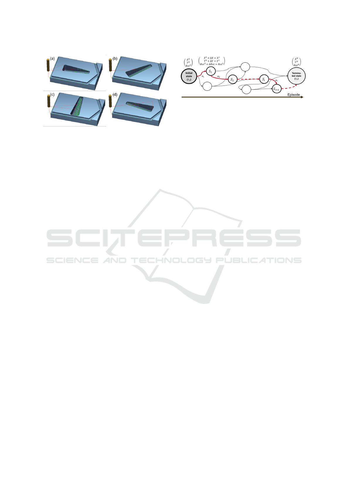
Figure 1: Examples of the Shape of the WP with Slot An-
gles (SA) (a) 0
◦
(B) 45
◦
(C) 90
◦
(C) 180
◦
.
the following state (S
0
) in an MDP is dependent only
on the current state (S) and action (a) pair.
The RL agent can optimise the WP clamping po-
sition by iteratively changing the WP position in the
work space of the milling machine. After a prede-
fined number of WP position changes is conducted,
the optimisation process is terminated. The last posi-
tion before the termination is considered to be the fi-
nal WP position proposed by the agent. Such a cycle
from random initialisation of the WP position to the
termination of the optimisation process is called an
episode. A number of allowed WP position changes
within the episode is referred to as a number of steps
within an episode.
The addressed task is non-stochastic, meaning that
a certain action (a) in a given state (S) will always
result in the same following state (S
0
). The clamp-
ing position problem is designed as a sequential deci-
sion making process with a finite number of steps (i)
within an episode and with the goal, that the trained
agent finds a near-optimal position within a few steps.
3.2.1 State-Action Representation
At every optimisation step the RL agent is allowed to
move the WP in the X and Y-axis directions, as well
as to rotate the WP. The magnitude of the changes
made to the WP position at each optimization step is
controlled by the action of the RL agent. Undertaken
step sizes can range from zero up to the allowed maxi-
mum limit. In our experiments we limit the maximum
single move along X and Y-axis to 40 mm. The max-
imum step size for the rotation angle is equal to 35
◦
.
The agent’s current state plus the action de-
fines the new clamping position of the WP,
with which the milling process simulation is ex-
ecuted. This is summarised in Figure 2, such
that the WP is initially placed within the work
space at (X
0
, Y
0
, RotationAngle
0
). At each step
(i) the RL agent incrementally moves the WP
by (∆X, ∆Y, ∆RotationAngle) into a new position
Figure 2: Formalisation of the Clamping Position Problem
as an MDP with Initial State, Intermediate States and Ter-
minated State within One Episode.
(X
i+1
, Y
i+1
, RotationAngle
i+1
), with which the simu-
lation is executed again and a feedback is given back
to the RL agent. This feedback states how much of
an improvement the change brought to the overall
milling performance in terms of avoiding axis colli-
sions, optimising the total traveled distance and min-
imising acceleration over all machine axes in the form
of reward (R
i
).
The observation space consists of eleven di-
mensions. Firstly, features describing the WP
clamping position in the machine working space
(X, Y, Rotation Angle), the current WP geometry
(Slot Angle), as well as a number of process param-
eters captured during the milling process at the cho-
sen clamping position by the agent is included. These
process parameters are the integrals of the squared
accelerations in the X- and Y-axis directions (called
(e
X
, e
Y
) since they correspond to energy), total trav-
eled distances in the X- and Y-axis directions (d
X
, d
Y
)
and indicators of reaching axis limits and axis colli-
sions (limit X, limit Y ). Lastly, we introduce the num-
ber of steps left within an episode before termina-
tion (steps left) as an additional input, as proposed by
(Pardo et al., 2018). This helps the agent to determine
whether it can reach a certain point in the working
space with the steps left in the episode and is espe-
cially beneficial if the number of steps allowed within
an episode is small. The final input is a tuple defined
as (X, Y, Rotation Angle, Slot Angle, d
X
, d
Y
, e
X
, e
Y
,
limit X, limit Y, steps left).
3.2.2 Reward Function
A reward function is required for the RL agent to
guide it through the optimisation process. It incen-
tivises the RL agent to learn the optimal clamping po-
sition. Higher rewards result from the minimisation
of accelerations and travelled distances. All observa-
tions have to be combined into a total reward. The fol-
lowing equations invert the observations (lower val-
ues correspond to higher rewards) and normalises
them:
ICEIS 2020 - 22nd International Conference on Enterprise Information Systems
508

e
X, norm
= (e
X, max
− e
X
)/(e
X, max
− e
X, min
) (1)
e
Y, norm
= (e
Y, max
− e
Y
)/(e
Y, max
− e
Y, min
) (2)
d
X, norm
= (d
X, max
− d
X
)/(d
X, max
− d
X min
) (3)
d
Y, norm
= (d
Y, max
− d
Y
)/(d
Y, max
− d
Y, min
) (4)
where:
e
.,norm
– normalised values for the integrated squared
accelerations along the X- and Y-axis
e
.,min
, e
.,max
– minimum and maximum values for e
X
and e
Y
d
.,norm
– normalised values for the travelled distances
along the X- and Y-axis
d
.,min
, d
.,max
– minimum and maximum values for d
X
and d
Y
For the considered machine, the X-axis is heavier than
the Y-axis. Therefore, e
X,norm
and d
X,norm
is weighted
higher than e
Y,norm
and d
Y,norm
in the combined reward
components e and d:
e = 2e
X, norm
+ e
Y, norm
(5)
d = 2d
X, norm
+ d
Y, norm
(6)
The total reward after every action is a combination
of the acceleration related term e from eq. (5) and the
distance related term d from eq. (6), such that:
R
i
=
(
0.7e + 0.3d no axis collision
−1 axis collision
(7)
The weights in eq. (7) give a higher importance to
the acceleration term e than to the distance term d,
because accelerations also cause disturbances in the
machining process. When an axis collision occurs
a reward of −1 is immediately awarded. The tuples
for the state-action-reward representation are briefly
summarised in Table 1.
Table 1: Summary of the Main Parameters of the Optimisa-
tion Task Formalised as an MDP.
State
(X, Y, Rotation Angle, Slot Angle, d
X
,
d
Y
, e
X
, e
Y
, limit X, limit Y, steps left)
Action (∆X, ∆Y, ∆Rotation Angle)
R
i
= 0.7e + 0.3d
Reward e = 2e
X,norm
+ e
Y,norm
d = 2d
X,norm
+ d
Y,norm
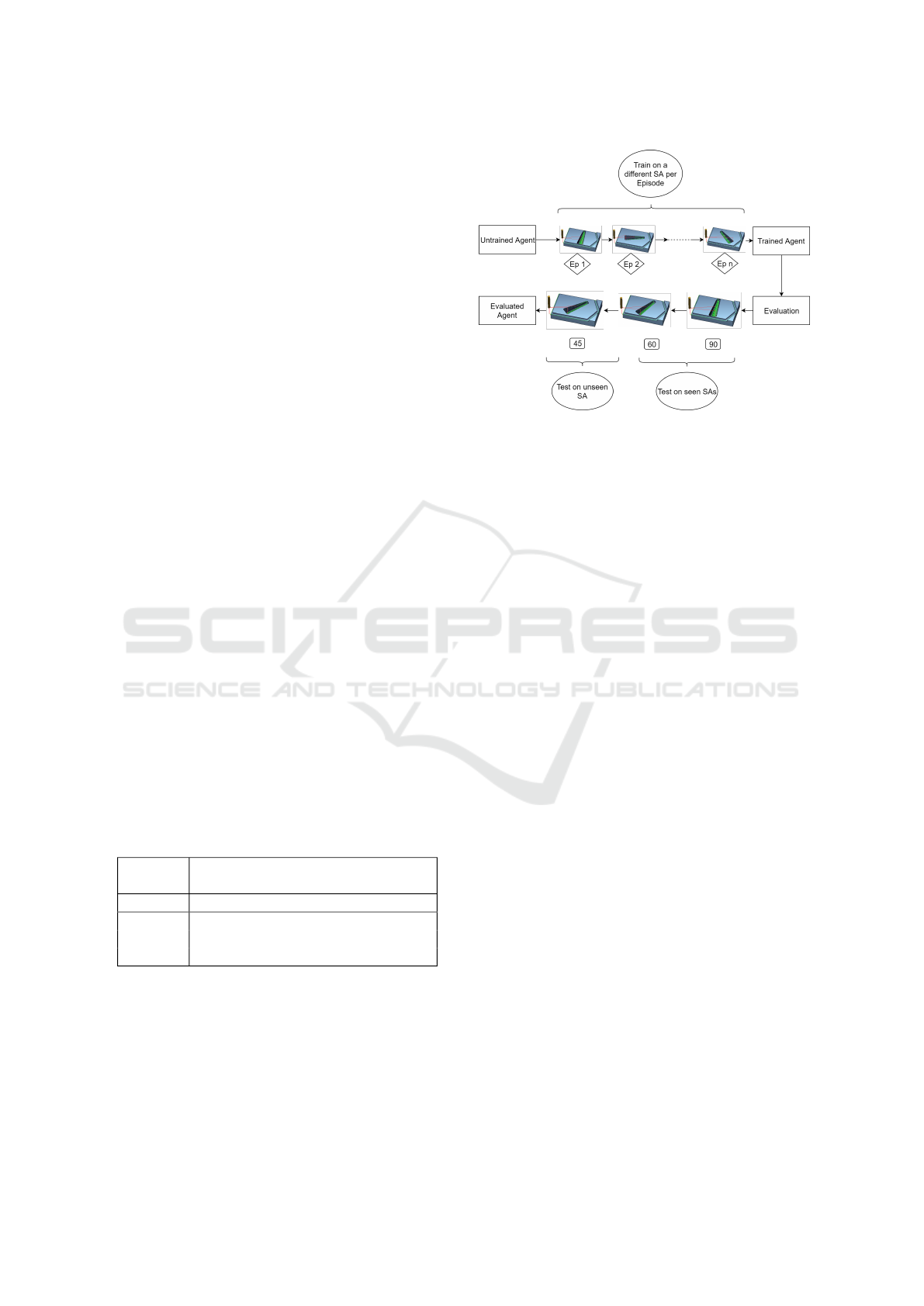
3.3 RL Agent Training and Validation
While learning the WP position optimisation strategy
the RL agent conducts a number of training episodes.
The training and evaluation process employed in this
study is summarised in Figure 3. At the start of each
episode a new WP geometry is generated and the WP
Figure 3: Training and Evaluation Process of the RL Agent.
position is randomly initialised. WP geometry stays
unchanged within one episode. During training the
RL agent encounters various WP geometries (slot an-
gles (SA)) with the exception of the angles ranging
between 40
◦
and 50
◦
. The trained agent is evaluated
on an unseen WP with the slot angle of 45
◦
. This
allows to determine if the given RL agent is not over-
fitting to solutions seen during the training, but learns
a generic optimisation strategy capable of interpreting
and solving unseen WP geometries.
Since the last WP position within an episode is
considered to be the final solution, the last reward in
an episode is an important metric. It provides an indi-
cation whether the agent found the optimal clamping
position. A trained RL agent is considered to be ca-
pable of generalisation if it can find a near-optimal
clamping position for an unseen WP with no addi-
tional learning within one episode.
The WP optimisation task is implemented as an
OpenAI Gym environment (Brockman et al., 2016).
We use the SAC implementation from stable baselines
(Hill et al., 2018) for solving the optimisation task in
the created environment. All training and evaluation
is conducted in docker containers (Merkel, 2014) to
ensure the independence of the experiments from the
used software and hardware. Each RL setup is in-
dependently trained and evaluated three times with
three fixed random seeds shared across all experi-
ments. This allows to evaluate and compare not only
the final performance, but also the stability of learning
while ensuring the reproducibility of the results.
3.3.1 Approximation of the Simulation with
Machine Learning
The training environment for the RL agent is a
SinuTrain simulation incorporating various WP ge-
ometries and machine kinematics. Depending on the
Using Reinforcement Learning for Optimization of a Workpiece Clamping Position in a Machine Tool
509

task, a SinuTrain simulation takes at least 4 seconds
for a successful run and 1 second for a failed run. In
this case a failed run would refer to an axis collision
and early termination of the run. During the train-
ing process thousands of interactions between the RL
agent and the simulation may be required, which re-
sults in impractically long training times. A consider-
ably faster environment for RL agent testing is created
to mimic the SinuTrain simulation with a combination
of machine learning (ML) models. These models pre-
dict simulation outcomes for a given set of input pa-
rameters. The steps to building these ML models are
data generation, ML-ensemble creation for prediction
and ML-ensemble training and validation.
3.3.2 Data Generation
Predictive models approximating the milling process
behaviour have to be built from the SinuTrain sim-
ulation runs with a set of input parameters (X, Y ,
Rotation Angle, Slot Angle) that covers the entire pa-
rameter space. These parameters are generated ac-
cording to randomised design. Random sampling
achieves good performance for large sample counts
(Garud et al., 2017). In total 180000 points are gener-
ated.
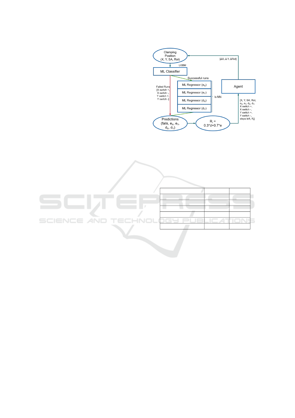
3.3.3 ML Ensemble for Prediction
The ML models are structured as a waterfall of a clas-
sifier, followed by a set of regression models. Fig-
ure 4 provides an overview of the ML-ensemble ar-
chitecture used to mimic the functioning of a 3-axis
milling machine. The classifier has the purpose of
determining whether a given WP position in the ma-
chine space would cause an axis collision during the
milling process or complete successfully, and further-
more returns the corresponding error message. These
error messages contain the axis of the machine that
caused the collision and whether it was in the positive
or negative direction of movement.
Only the set of inputs that will lead to success-
ful runs are propagated further to the regression mod-
els. Four regression models are trained to predict the
e
X
, e
Y
, d
X
, d
Y
values (defined in section 3.2.1) during
the WP processing. These values are used as input to
the RL agent and to calculate the reward.
3.3.4 ML-Ensemble Training and Validation
Ten-fold cross-validation (CV) is used to validate the
ML models (Kohavi, 1995). The data is split into ten
equal parts, nine parts are joined together and used as
the training set and the tenth part is used as the vali-
dation set. This process is repeated until each of the
Figure 4: Architecture of the ML-Ensemble. A Classifier
Predicts If the Simulation with the given Input Parameters
Is Going to Fail or Run Successfully. In the Case of a Pos-
itive Result, Regression Models Predict Output Parameters
(One Model per Parameter). Gradient Boosting, with a De-
gree of 2 Polynomial Feature Basis Expansion, Is Used as
a Classifier and K-Nearest Neighbors (K-NN), with k = 75
and Uniform Weighting, Is Used for the Regression Models.
Table 2: Summary of the Classifier Accuracy.
F1-Score Totals
Success 0.990 34943
Limit X + 0.949 4200
Limit X - 0.901 36608
Limit Y + 0.960 16892
Limit Y - 0.932 46730
Weighted Average 0.942 139373
parts was used once as the validation set and each rep-
etition of the process is called a CV-fold. This process
ensures that there is never any overlap between the
training and the validation data. For each of the folds
a prediction accuracy is calculated, and the average of
these accuracies is returned as the final performance
evaluation of the ML model.
The accuracy of the classifier is determined by
the weighted F1-score, as it is important to have
good performance in the prediction of each of the
classes. Table 2 summarises the F1-score for each
of the classes and the overall classification is evalu-
ated by a weighted average according to the sizes of
the different classes. This overall F1-score is 94.2%
and the fact that 99% of the successful runs are cor-
rectly identified means that the regression models re-
ceive the information they need to make accurate pre-
dictions.
For the regression models, the R-squared metric
is used to compare models and to choose the opti-
mal model. The R-squared value for each regression
ICEIS 2020 - 22nd International Conference on Enterprise Information Systems
510

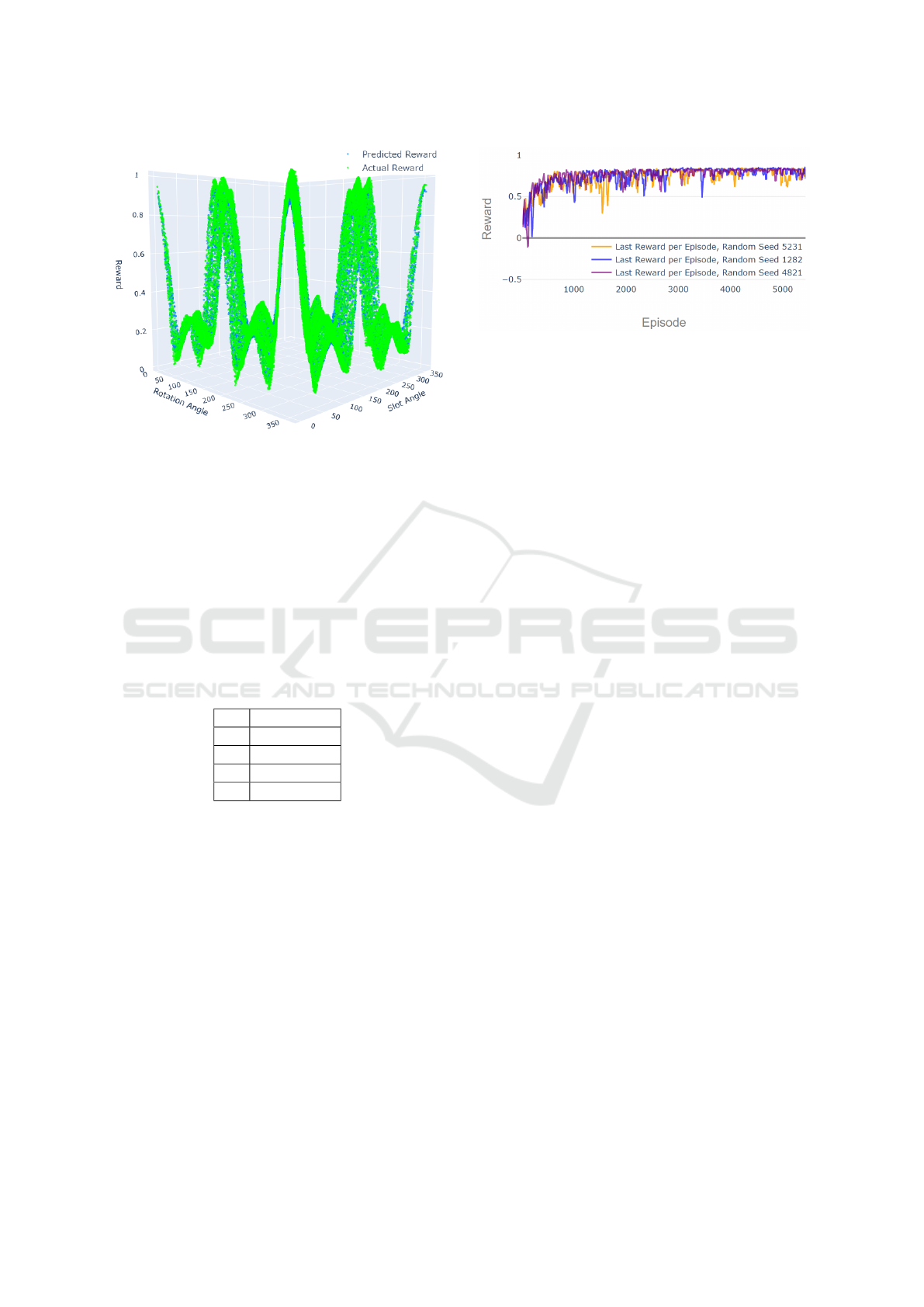
Figure 5: Predicted versus Actual Rewards for Successful
Simulation Runs.
model is quoted in Table 3 and Figure 5 depicts the re-
ward surface comparing predicted and actual rewards.
The reward surface represents only the part of eq. (7)
corresponding to no axis collisions and is a combina-
tion of the predictions for e
X
, e
Y
, d
X
, d
Y
. These pre-
dictions are summarised as described in section 3.2.2.
The deviation of the predicted values from the ac-
tual values are almost negligible, therefore the surface
produced by the ML-ensemble is a good representa-
tion of the true surface.
Table 3: Summary of the Regression Models Accuracy.
R-Squared
e
X
0.951
e
Y
0.947
d
X
0.840
d
Y
0.835
The resulting ML-ensemble can predict the outcome
of any simulation iteration under 0.01 seconds. This
offers up to a 400-fold improvement in the training
speed of the chosen RL algorithms.
4 EXPERIMENTAL RESULTS
The training of the RL agent is conducted on various
WP geometries and validated on two seen WP geome-
tries (slot angle of 90
◦
and 60
◦
) and an unseen WP
geometry (slot angle of 45
◦
) as described in section
Section 3. It tests whether the RL agent ”remembers”
good solutions seen during the training without over-
fitting to them and whether it can generalise to unseen
WPs.
Figure 6: Last Reward per Episode during Training,
Episode Length - 110 Steps, Total Training Steps - 600.000.
Firstly, we investigate if the RL agent is capable of
finding an optimal clamping position for an unseen
WP within 110 steps per episode. It is a fairly large
number of steps which allows the RL agent to conduct
more exploration and recover from mistakes, such as
not heading straight to the optimal point from the be-
ginning of an episode.
Figure 6 and Figure 7 show the last reward per
episode, with a smoothing window of 30 episodes,
during training and validation respectively. The RL
agent is trained over 600.000 steps before the valida-
tion starts. The three lines of different colours rep-
resent the achieved last reward per episode for inde-
pendent training (white background area) and valida-
tion (the light-grey background area for the 90
◦
slot
angle, the grey background area for the 60
◦
slot angle
and the dark-grey background area for the 45
◦
slot an-
gle) runs with different random seeds. The maximum
possible reward depends on the slot angle because of
the implicit differences in the milling process. This
explains the changes in general reward level seen at
different validation stages for each slot angle. At all
validation runs the RL agent never gets negative re-
wards at the last episode step. It proves that the RL
agent learns how to avoid axis collisions for differ-
ent initialisation positions across the whole machine
space. Moreover, the last reward per episode stays
close to the maximum for both seen WP configura-
tions with 90
◦
and 60
◦
slot angles, as well as for the
unseen 45
◦
configuration. The RL agent is capable of
consistently placing the WP with an unseen geometry
in positions close to the optimum.
Figure 8 shows position changes of the WP in
the three-dimensional space of (X, Y, Rotation Angle)
at each optimisation step over some randomly sam-
pled validation episodes from all three independently
trained RL agents. This allows for understanding of
the actions of the RL agent and to validate if the
learned strategy optimally solves the task. We pro-
vide the visualisation only for the WP with a 45
◦
slot
angle, since understanding the generalisation capabil-
Using Reinforcement Learning for Optimization of a Workpiece Clamping Position in a Machine Tool
511

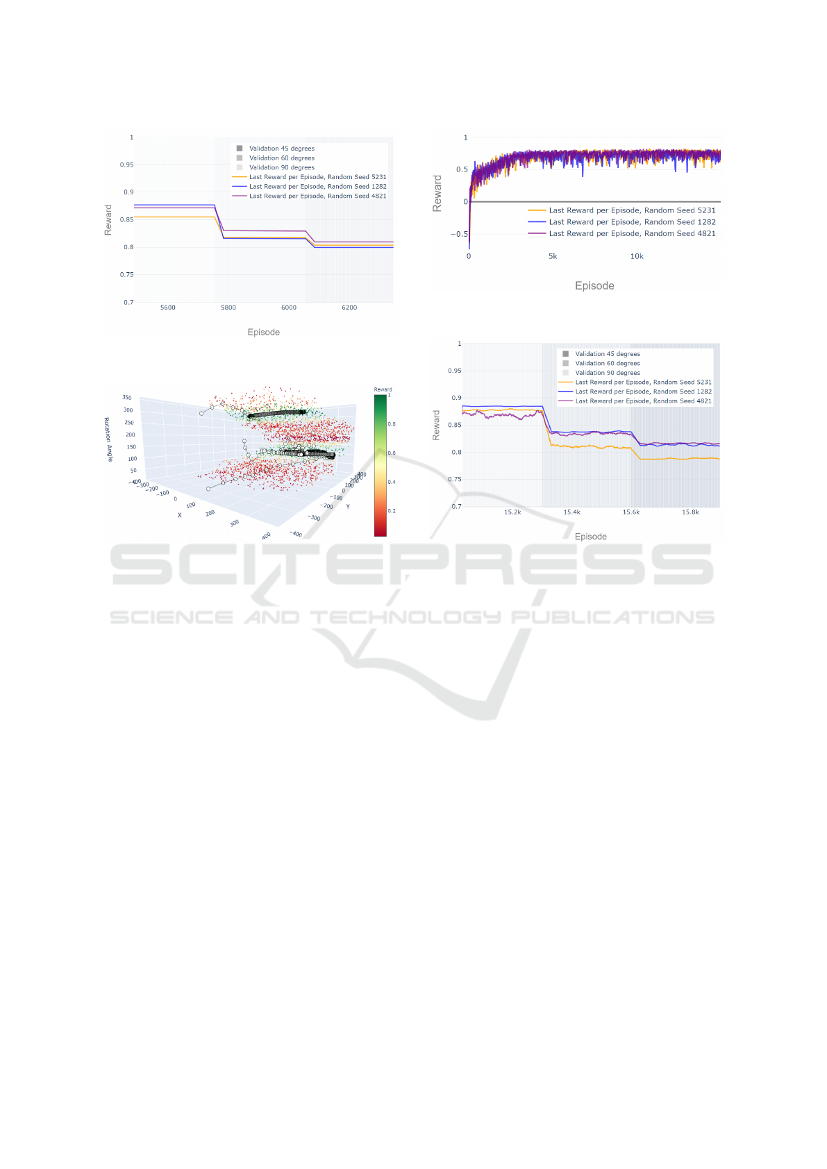
Figure 7: Last Reward per Episode during Validation,
Episode Length - 110 Steps, Total Training Steps - 600.000.
Figure 8: Moves of the RL Agents (110 Steps per Episode)
in the Machine Space. The Episode Trajectories Are Ran-
domly Sampled across the Three Trained RL Agents.
ities of the RL agent is the main purpose of this study.
One connected line in the figure corresponds to one
optimisation episode. Points show positions of the
WP in the machine working space, while lines depict
the transitions following the RL agent’s chosen ac-
tions. The colour of the points is changing gradually
from white to black throughout the episode such that
the start and end points can easily be recognised. The
cloud of points represents the area where the milling
process runs through without axis collisions and the
empty space surrounding the point cloud represents
the WP positions where the simulation fails to run.
The colour of every point in the cloud encodes the
reward for placing the WP in the given position. It
can be seen, that across all initialisation points the RL
agent first moves the WP out of the axis collision area
in the shortest possible way to minimise the penalty.
Afterwards, it gradually moves the WP towards one
of the two optimal areas with the highest rewards. As
soon as the high reward area is achieved the RL agent
significantly decreases the step-size and stays within
the high-reward area.
Looking at Figure 8, the RL agent mostly needs
a small fraction of the available steps to reach areas
of high reward. The overall goal is to find an optimal
Figure 9: Last Reward per Episode during Training,
Episode Length - 20 Steps, Total Training Steps - 300.000.
Figure 10: Last Reward per Episode during Validation,
Episode Length - 20 Steps, Total Training Steps - 300.000.
WP clamping position while keeping the number of
iteration steps at a minimum. Therefore we reduce the
number of steps per episode to 20. This requires the
agent to deviate as little as possible from the direction
of the optimal point during the episode, in order to
reach it before or at the last step.
With 20 steps per episode, up to 300.000 train-
ing steps are required to achieve the best result (Fig-
ure 9). This can be explained by the fact that the RL
agent does not need to learn to stay in the area of high
reward for many steps before the termination of the
episode. At the same time, longer training leads to a
slight performance decrease.
Figure 10 shows that three independently trained
RL agents have higher differences in the final per-
formance comparing to the 110 steps per episode RL
agents. This points towards less stable training. Dur-
ing two training runs the RL Agents were able to learn
optimal solutions for all three validation slot angles.
Depending on the initialisation point, the RL Agent
does not always move the WP into the same place
as for 110 steps per episode. Nevertheless, all cho-
sen points are very close to the optimum. The third
trained RL agent underperforms on all three valida-
tion angles.
ICEIS 2020 - 22nd International Conference on Enterprise Information Systems
512

Figure 11: Moves of the RL Agents (20 Steps per Episode)
in the Machine Space. The Episode Trajectories Are Ran-
domly Sampled across the Three Trained RL Agents.
The learned optimisation strategy is visualised in Fig-
ure 11. Similarly to the case with 110 steps per
episode, the RL agent moves the WP out of the axis
collision area in big steps first and then gradually ap-
proaches the optimal points.
A further decrease of the training steps per episode
leads to a decrease of the stability of the results be-
cause depending on the WP initialisation point, the
RL agent may not always be capable of reaching the
optimal point.
5 CONCLUSION AND OUTLOOK
We formalised the problem of finding an optimal WP
clamping position as an MDP problem, set up a train-
ing environment for an RL agent using an approxima-
tion of the SinuTrain milling simulation with stacked
ML models and successfully demonstrated that an
RL agent can solve the WP clamping position opti-
misation task. Through a number of evaluations we
demonstrated that a trained RL agent is capable of
generalisation to new, previously unseen (but simi-
lar in geometry) WPs. In the case of a 3-axis ma-
chine tool, it is capable of finding a valid and near-
optimal clamping position within a limited number
of optimisation steps for an unseen WP without ad-
ditional training when the WP geometry is explicitly
described as a part of the state space.
This paper is a proof-of-concept work demonstrat-
ing that RL can be applied in complex optimisation
tasks from the field of mechanical engineering, such
as the search for an optimal WP clamping position.
In this study, we elaborated only on a simple 3-axis
milling machine use case. In future work, the demon-
strated results can be transferred to more complex
WPs requiring processing on a 5-Axis milling ma-
chine. Another important aspect of the possible fu-
ture research focuses on a solution able to handle
a variety of WPs, without providing a set of hand-
crafted features describing the WP. For example, we
can define the optimisation task as a Partially Observ-
able Markov Decision Process (POMDP) where WP
related features can be learned indirectly by the RL
agent through simulation feedback at the beginning
of the optimisation process. Possible solutions for
such a POMDP optimisation task includes the use of
frame stacking, RL with Recurrent Neural Networks
or a meta-learning method. To progress further in the
direction of a production capable solution, we would
need to improve the RL training efficiency and trans-
ferability of RL-learned solutions to new WPs and
machine tools with complex axis movements with no
or little extra training required.
REFERENCES
Anderson, R. L. (1953). Recent advances in finding best op-
erating conditions. Journal of the American Statistical
Association, 48(264):789–798.
Baer, S., Bakakeu Romuald Jupiter, Meyes Richard, and
Meisen Tobias (25.09.2019-27.09.2019). Multi-agent
reinforcement learning for job shop scheduling in flex-
ible manufacturing systems. In 2019 Second Interna-
tional Conference on Artificial Intelligence for Indus-
tries (AI4I). IEEE.
Bakakeu, J., Tolksdorf, S., Bauer, J., Klos, H.-H., Peschke,
J., Fehrle, A., Eberlein, W., B
¨
urner, J., Brossog, M.,
Jahn, L., and Franke, J. (2018). An artificial intel-
ligence approach for online optimization of flexible
manufacturing systems. Applied Mechanics and Ma-
terials, 882:96–108.
Bello, I., Pham, H., Le, Q. V., Norouzi, M., and Bengio, S.
(2016). Neural combinatorial optimization with rein-
forcement learning. arXiv preprint arXiv:1611.09940.
Brockman, G., Cheung, V., Pettersson, L., Schneider, J.,
Schulman, J., Tang, J., and Zaremba, W. (2016). Ope-
nai gym.
Garud, S. S., Karimi, I. A., and Kraft, M. (2017). Design
of computer experiments: A review. Computers and
Chemical Engineering.
Haarnoja, T., Zhou, A., Abbeel, P., and Levine, S. (2018).
Soft actor-critic: Off-policy maximum entropy deep
reinforcement learning with a stochastic actor.
Hajela, P. and Lin, C.-Y. (1992). Genetic search strategies
in multicriterion optimal design. Structural Optimiza-
tion, 4(2):99–107.
Hill, A., Raffin, A., Ernestus, M., Gleave, A., Kanervisto,
A., Traore, R., Dhariwal, P., Hesse, C., Klimov, O.,
Nichol, A., Plappert, M., Radford, A., Schulman, J.,
Sidor, S., and Wu, Y. (2018). Stable baselines.
Howard, R. A. (1960). Dynamic programming and markov
processes.
Johannink, T., Bahl, S., Nair, A., Luo, J., Kumar, A.,
Loskyll, M., Ojea, J. A., Solowjow, E., and Levine,
S. (20.05.2019 - 24.05.2019). Residual reinforcement
learning for robot control. In 2019 International Con-
Using Reinforcement Learning for Optimization of a Workpiece Clamping Position in a Machine Tool
513

ference on Robotics and Automation (ICRA), pages
6023–6029. IEEE.
Kohavi, R. (1995). A study of cross-validation and boot-
strap for accuracy estimation and model selection.
Kool, W., van Hoof, H., and Welling, M. (2018). Atten-
tion, learn to solve routing problems! arXiv preprint
arXiv:1803.08475 In Citavi anzeigen.
Li, K. and Malik, J. (2016). Learning to optimize.
Li, K. and Malik, J. (2017). Learning to optimize neural
nets.
Merkel, D. (2014). Docker: lightweight linux containers for
consistent development and deployment. Linux jour-
nal, 2014(239):2.
Nazari, M., Oroojlooy, A., Snyder, L., and Tak
´
ac, M.
(2018). Reinforcement learning for solving the ve-
hicle routing problem. In Advances in Neural Infor-
mation Processing Systems, pages 9839–9849.
Pardo, F., Tavakoli, A., Levdik, V., and Kormushev, P.
(2018). Time limits in reinforcement learning. In
Dy, J. and Krause, A., editors, Proceedings of the
35th International Conference on Machine Learning,
volume 80 of Proceedings of Machine Learning Re-
search, pages 4045–4054, Stockholmsm
¨
assan, Stock-
holm Sweden. PMLR.
Sutton, R. S. and Barto, A. (2018). Reinforcement learning:
An introduction. Adaptive computation and machine
learning. The MIT Press, Cambridge, MA and Lon-
don, second edition edition.
van Laarhoven, P. J. M. and Aarts, E. H. L. (1987). Simu-
lated annealing. In van Laarhoven, P. J. M. and Aarts,
E. H. L., editors, Simulated Annealing: Theory and
Applications, pages 7–15. Springer Netherlands, Dor-
drecht.
Vinyals, O., Babuschkin, I., Czarnecki, W. M., Mathieu,
M., Dudzik, A., Chung, J., Choi, D. H., Powell, R.,
Ewalds, T., Georgiev, P., Oh, J., Horgan, D., Kroiss,
M., Danihelka, I., Huang, A., Sifre, L., Cai, T., Aga-
piou, J. P., Jaderberg, M., Vezhnevets, A. S., Leblond,
R., Pohlen, T., Dalibard, V., Budden, D., Sulsky, Y.,
Molloy, J., Paine, T. L., Gulcehre, C., Wang, Z.,
Pfaff, T., Wu, Y., Ring, R., Yogatama, D., W
¨
unsch,
D., McKinney, K., Smith, O., Schaul, T., Lillicrap,
T., Kavukcuoglu, K., Hassabis, D., Apps, C., and
Silver, D. (2019). Grandmaster level in starcraft ii
using multi-agent reinforcement learning. Nature,
575(7782):350–354.
ICEIS 2020 - 22nd International Conference on Enterprise Information Systems
514