Predicting e-Mail Response Time in Corporate Customer Support

Anton Borg

1 a

, Jim Ahlstrand

and Martin Boldt

1 b

Blekinge Institute of Technology, 37179 Karlskrona, Sweden

Telenor AB, Karlskrona, Sweden

Keywords:

e-Mail Time-to-Respond, Prediction, Random Forest, Machine Learning, Decision Support.

Abstract:

Maintaining high degree of customer satisfaction is important for any corporation, which involves the customer

support process. One important factor in this work is to keep customers’ wait time for a reply at levels that are

acceptable to them. In this study we investigate to what extent models trained by the Random Forest learning

algorithm can be used to predict e-mail time-to-respond time for both customer support agents as well as

customers. The data set includes 51, 682 customer support e-mails of various topics from a large telecom

operator. The results indicate that it is possible to predict the time-to-respond for both customer support

agents (AUC of 0.90) as well as for customers (AUC of 0.85). These results indicate that the approach can be

used to improve communication efﬁciency, e.g. by anticipating the staff needs in customer support, but also

indicating when a response is expected to take a longer time than usual.

1 INTRODUCTION

An important element in any corporation is to main-

tain high-quality and cost-efﬁcient interaction with

the customers. This is especially important for in-

teractions between the organization and customer via

customer support, since failing to resolve customers

issues satisfactorily risk negatively affecting the cus-

tomers view of the organization. Further, in a prolon-

gation this might affect the overall reputation of the

organization. In highly competitive markets, a single

negative customer service experience can deter poten-

tial new customers from a company or increase the

risk of existing customers to drop out (Halpin, 2016),

both negatively affecting the volume of business.

For many customers e-mails still account for

an important means of communication due to both

its ease and widespread use within almost all age

groups (Kooti et al., 2015). As such, implementing

efﬁcient customer service processes that target cus-

tomer e-mail communication is a necessity for cor-

porations as they receive large numbers of such cus-

tomer service e-mails each day. Furthermore, the cus-

tomers expect short response times to digital mes-

sages, which further complicates the customer service

process (Church and de Oliveira, 2013).

https://orcid.org/0000-0002-8929-7220

https://orcid.org/0000-0002-9316-4842

In this study we investigate the possibility to use

supervised machine learning in order to predict when

an e-mail response will be received, time-to-respond

(TTR) or responsiveness. The semi-automated cus-

tomer service e-mail management system studied ex-

ists within one of the bigger telecom operators in Eu-

rope with over 200 million customers worldwide, and

some 2.5 million in Sweden. When these customers

experience problems they often turn to e-mail as their

means of communication with the company, by sub-

mitting an e-mail to a generic customer service e-mail

address. Under-stafﬁng might impact the efﬁciency of

customer support, negatively impacting customer re-

lations. However, while over-stafﬁng might produce

quick responses, it might also result in customer sup-

port agents being idle. Consequently, it is important

to be able to predict the customer support workload in

order to successfully schedule personnel and improve

communication efﬁciency (Yang et al., 2017).

Customer service e-mails, provided by the tele-

com company, contains support errands with differ-

ent topics. Each customer service e-mail might con-

tain different topics, and the importance of each topic

might be of varying importance, depending on the

customer. Different topics require different actions

by customers, and thus would require varying time

before a response can be expected. The content of an

e-mail within a topic, e.g. invoice, might also affect

time-to-respond, as certain actions are more compli-

Borg, A., Ahlstrand, J. and Boldt, M.

Predicting e-Mail Response Time in Corporate Customer Support.

DOI: 10.5220/0009347303050314

In Proceedings of the 22nd International Conference on Enterprise Information Systems (ICEIS 2020) - Volume 1, pages 305-314

ISBN: 978-989-758-423-7

305

cated than others. Further, a customer service e-mail

might contain two paragraphs of text, one detailing

a technical issue, and the other one an order errand.

As such, the e-mail topic would be sorted as Invoice,

TechicalIssue, and Order. This would further affect

response time.

1.1 Aims and Objectives

In this study we investigate the possibility to predict

the time-to-respond for received e-mails based on its

content. If successful, it would be possible to adjust

the schedules for customer support personnel in or-

der to improve efﬁciency. The two main questions

investigated in this work are as follows. First, to what

extent it is possible to predict the time required by

customer support agents to respond to e-mails. Sec-

ond, to what extent it is possible to predict the time it

takes customers to respond to e-mails from customer

support personnel.

1.2 Scope and Limitations

The scope of this study is within a Swedish setting,

involving e-mail messages written in Swedish sent to

the customer service branch of the studied telecom

company. However, the problem studied is general

enough to be of interest for other organizations as

well. In this study, e-mails where no reply exists have

been excluded, as it has been suggested to be a sep-

arate classiﬁcation task (Huang and Ku, 2018). Fur-

ther, time-to-respond (TTR) is investigated indepen-

dent of the workload of agents, and the content of the

e-mails.

2 RELATED WORK

Time-to-Respond, or responsiveness, can affect the

perceived relationship between people both posi-

tively and negatively (Church and de Oliveira, 2013),

(Avrahami and Hudson, 2006), (Avrahami et al.,

2008).

Investigations into mobile instant messaging (e.g.

SMS) indicates that it is possible to predict whether a

user will read a message within a few minutes of re-

ceiving it (70.6% accuracy) (Pielot et al., 2014). This

can be predicted based on only seven features, e.g.

screen activity, or ringer mode.

Responsiveness to IM has been investigated, and

been predicted successfully ( 90% accuracy) (Avra-

hami and Hudson, 2006). The paper where limited

to messages initiating new sessions, but the model

where capable of predicting whether an initiated ses-

sion would get a response within 30s, 1, 2, 5, or 10

minutes. Predicting the response time when inter-

acting with chatbots using IM have also been inves-

tigated, within four time intervals < 10s, 10 − 30s,

30 − 300s, and > 300s (Accuracy of 0.89), but also

whether a message will receive a response (Huang

and Ku, 2018).

Similarly to IM, response time in chat-rooms have

also been investigated, with one study ﬁnding that

the cognitive and emotional load affect response time

within and between customer support agents (Rafaeli

et al., 2019). In a customer support setting, the cogni-

tive load denotes e.g. the number of words or amount

of information that must be processed. TTR predic-

tions have also been investigated in chat rooms (AUC

0.971), intending to detect short or long response

times (Ikoro et al., 2017).

However, it seems that there is little research that

have investigated predicting the TTR of e-mails in a

customer support setting. This presents a research gap

as it has been argued that e-mails are a distinct type

of text compared to types of text (Baron, 1998). Re-

search indicates that it is possible to estimate the time

for an e-mail response to arrive, within the time inter-

vals of < 25 min, 25 − 245 min, or > 245 min (Yang

et al., 2017). Similarly, research has been conducted

on personal e-mail (i.e. non-corporate) (Kooti et al.,

2015). However, this investigates quite small TTRs

which, although suitable for employee e-mails, might

not conform to the customer support setting according

to domain experts. Further, the workload estimation

of customer support agents work resolution beneﬁts

from an increased resolution, i.e. more bins.

3 DATA

The data set consists of 51, 682 e-mails from the cus-

tomer service department from a Swedish branch of

a major telecom corporation. Each e-mail consists of

the:

• subject line,

• send-to address,

• sent time, and

• e-mail body text content.

Each e-mail is also labeled with at least one label. In

total there exists 36 distinct topic labels, each inde-

pendent from the others, where several of these might

be present in any given e-mail. The topics have been

set by a rule-based system that was manually devel-

oped, conﬁgured and ﬁne-tuned over several years by

domain expertise within the corporation.

ICEIS 2020 - 22nd International Conference on Enterprise Information Systems

306

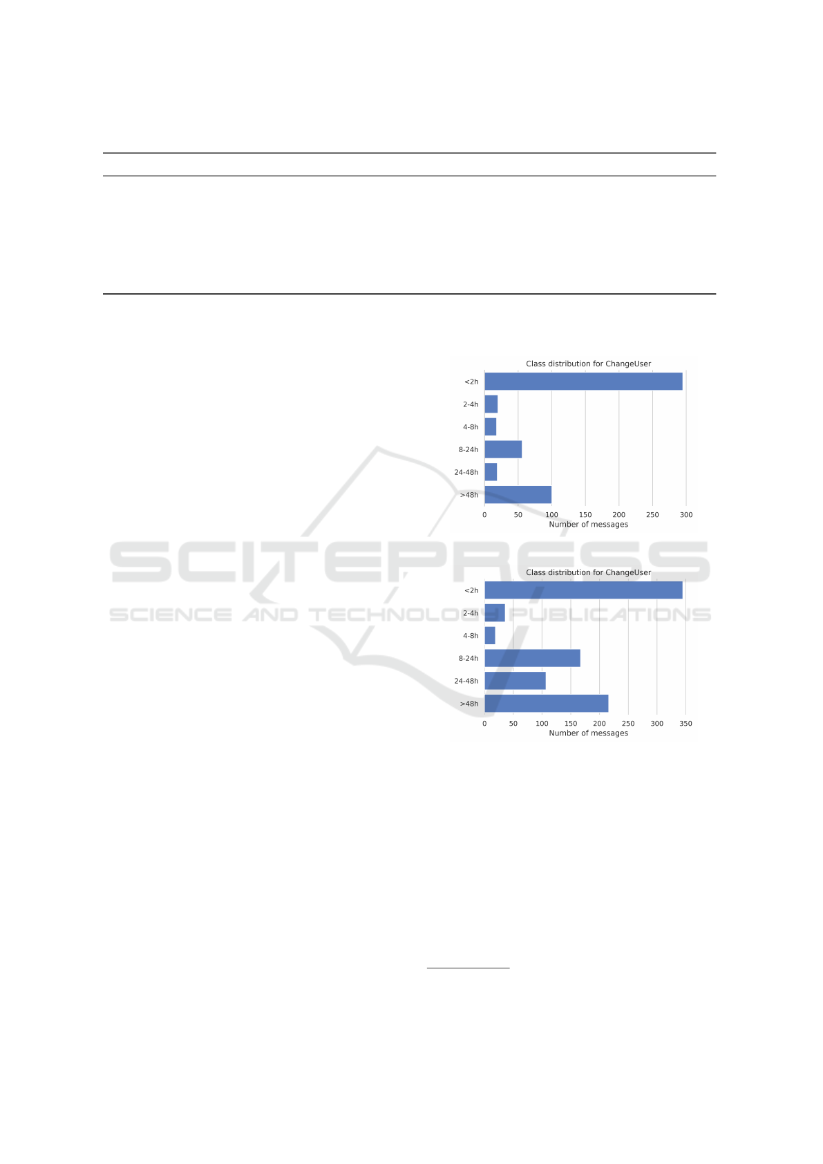
Table 1: Description of the Features Extracted or Calculated from the Data Set.

Feature name Type Value range Description

Text sentiment Float [−1, +1] Text sentiment of an e-mail ranging negative to positive.

Customer escalated Boolean {0, 1} Whether customer changed between messages in thread.

Agent escalated Boolean {0, 1} Whether agent changed between messages in thread.

Old Boolean {0, 1} Whether a message is older than 48 hours, or not.

Text complexity Float [0, 100] Indication of the text complexity.

Sender Categorical Text The e-mail address of the sender.

Message length Integer ≥ 1 Number of characters in each e-mail message.

A DoNotUnderstand topic label acts as the last re-

sort for any e-mail that the current labeling system

is unable to classify. Those e-mails have been ex-

cluded from the data set and each e-mail has been

anonymized. Further, ends of threads have been ex-

cluded from the data set (i.e. e-mails where no reply

exists), as that has been suggested to be a separate

classiﬁcation task (Huang and Ku, 2018).

The e-mails are grouped into conversation threads,

and for each e-mail the date and time sent is avail-

able, enabling the construction of a timeline for each

thread. Further, it is possible to shift the time-date

information in each thread by one step, so that the

future sent time is available for each e-mail in the

thread. As such, this data can be considered the TTR.

In order to adjust the resolution of the TTR, the date-

time where binned into groups (Avrahami and Hud-

son, 2006). The bins were decided by consulting

with the telecom company and thus using their do-

main knowledge. Six bins where utilized: response

within 2 hours, between 2 − 4 hours, between 4 − 8

hours, between 8 − 24 hours, between 24 − 48 hours,

and more than 48 hours. The bins are considered as

the class labels.

The data set is divided into subsets, by topic and

sender. The topics Credit (n = 6, 239), Order (n =

2, 221), and ChangeUser (n = 1, 398) are used to in-

vestigate this problem. Further, similar to the work

by Yang et al. each topic is divided into one set

for e-mails sent from the telecom corporation and an-

other set for e-mails sent by the customer (Yang et al.,

2017). In this case, the agents can be considered a

more homogeneous group (similar training and expe-

rience), whereas the customers could be regarded as

a heterogeneous group (different background and ex-

periences). As such, six data sets have been created.

The class distribution in the data set is exempli-

ﬁed by ChangeUser topic in Figure 1 for agents and

Figure 2 for customers. A majority of the messages

have a TTR within two hours, followed by a TTR

longer than 48 hours, 8 − 24 hours. A minority of

messages have a TTR between 2−4, 4−8, or 24−48

hours. Consequently, it would seem that messages get

responses ”immediately”, the next day, or after two

days.

Figure 1: ChangeUser Agent TTR Class Distribution.

Figure 2: ChangeUser Customer TTR Class Distribution.

3.1 Feature Extraction

For each e-mail in the data set, seven features are cal-

culated or extracted. A summary of all features used

in the study are shown in Table 1. First, Vader senti-

ment is used to calculate the Text sentiment for each e-

mail (Hutto and Gilbert, 2015), (Rafaeli et al., 2019).

As the primary language in this data set is Swedish, a

list of Swedish stop-words was used

. However, the

Swedish stop-words were extended by English stop-

words, as a fair amount of English also occurs due to

https://gist.github.com/peterdalle/8865eb918a824a475

b7ac5561f2f88e9

Predicting e-Mail Response Time in Corporate Customer Support

307

the corporate environment.

Second, for each message it was calculated

whether the customer or support agent responding

participating in the conversation had changed over

the thread timeline, denoted by the Boolean variables

Customer escalated and Agent escalated respectively.

A change in e.g. customer support agent indicates

the involvement of an agent experienced in the cur-

rent support errand. However, related work indicates

that as the number of participants increase, so do the

time to respond (Yang et al., 2017). The variable Old

denotes if the message has not received a response for

48 hours or more, as per internal rules at the company.

A Text complexity factor for the text is also calculated

as per

CF =

|{x}|

|x|

× 100, (1)

where x is the e-mail content (Abdallah et al., 2013).

Consequently, Equation 1 is the number of unique

words in the e-mail divided by the number of words

in the e-mail. A higher score indicates a higher com-

plexity in the text, which can affect the TTR (Rafaeli

et al., 2019). It should be noted that there exist differ-

ent readability scores for the English language, e.g.

Flesch–Kincaid score (Farr et al., 1951). However,

the applicability of these on Swedish text is unknown.

Finally, the Sender and Length of the e-mail is also in-

cluded as variables.

4 METHOD

This section describes the experimental approach,

which includes for instance the design and chosen

evaluation metrics.

4.1 Experiment Design

Two experiments with two different goals were in-

cluded in this study. The ﬁrst experiment aimed to

investigate whether it is possible to predict the time

a customer support agent would take to respond to

the e-mail received. As such, the experiment used the

data set containing e-mails sent by the customer and

tried to predict when the agent would respond. In this

experiment the independent variable was the models

trained by the learning algorithms described in Sec-

tion 4.2. The dependent variables were the evaluation

metrics described in Section 4.4, of which the AUC

metric was chosen as primary.

The second experiment is similar to the ﬁrst one,

but instead uses the data sets containing e-mails sent

by the customer support agents, thus aiming to predict

when the customer will respond. As such both the in-

dependent and the dependent variables were the same

as in the ﬁrst experiment.

Evaluation of the classiﬁcation performance was

handled using a 10-times 10-fold cross-validation

approach in order to train and evaluate the mod-

els (Flach, 2012). Each model’s performance was

measured using the metrics presented in Section 4.4.

4.2 Included Learning Algorithms

Random Forest (Breiman, 2001) was selected as the

learning algorithm to investigate in this study. It is a

suitable algorithm as the data contains both Boolean,

categorical, and continuous variables. Initially a SVM

model (Flach, 2012) was also evaluated, but since

Random Forest signiﬁcantly outperformed the SVM

models, they were excluded from the study. The rea-

son to why the SVM model showed inferior perfor-

mance is not clear. Although it is in line with the “No

free lunch” theorem, stating that no single model is

best in every situation. Thus, models’ performance

varies when evaluated over different problems.

The models trained by the Random Forest algo-

rithm were compared against a Random Guesser clas-

siﬁer using a uniform random guesser as baseline (Pe-

dregosa et al., 2011), (Yang et al., 2017).

4.3 Class-balance

In order to deal with the class imbalance of the dif-

ferent bins, a multi-class oversampling strategy was

used that relied on SMOTE and cleaned by removing

instances which are considered Tomek links (Batista

et al., 2003; Lema

ıtre et al., 2017). Using only over-

sampling can lead to over-ﬁtting of the classiﬁers as

majority class examples might overlap the minority

class space, and the artiﬁcial minority class exam-

ples might be sampled too deep into the majority class

space (Batista et al., 2003).

4.4 Evaluation Metrics

The models predictive performance in the experi-

ments were evaluated using standard evaluation met-

rics calculated based on the True Positives (TP), False

Positives (FP), True Negatives (TN), and False Neg-

atives (FN). The evaluation metrics consists of the

-score (micro average), Accuracy, and Area under

ROC-curve (AUC) (micro average).

The theoretical ground for these metrics are ex-

plained by Flach (Flach, 2012). The ﬁrst metric is

ICEIS 2020 - 22nd International Conference on Enterprise Information Systems

308

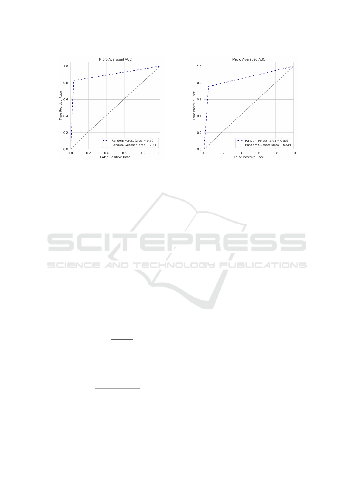
(a) Agent TTR Predictions. (b) Micro Averaged AUC for Agent Predictions (3a) and Cus-

tomer Predictions (3) over the Different Topics.

Figure 3: Customer TTR Predictions.

the traditional Accuracy that is deﬁned as in Equa-

tion 2 (Yang, 1999):

Acc =

T P + T N

T P + T N + FP +FN

(2)

It is a measurement of how well the model is capable

of predicting TP and TN compared to the total number

of instances. For the multi-class case, the accuracy

is equivalent to the Jaccard index. Accuracy ranges

between 0.0 − 1.0, where 1.0 is a perfect score.

However, in cases where there is a high number

of negatives, e.g. in a multi-class setting, accuracy is

not representative. In these cases the F

-score is often

used as an alternative, as it doesn’t take true negatives

into account (Flach, 2012). Similar to the Accuracy,

the F

-score ranges between 0.0 − 1.0, where 1.0 is

a perfect score. It is calculated as described in Equa-

tion 5, based on Equation 3 and Equation 4. In this

study micro-averaging was used as the number of la-

bels might vary between classes (Yang, 1999).

Precision =

T P

T P + FP

(3)

Recall =

T P

T P + FN

(4)

= 2 ∗

Precison ∗ Recall

Precision + Recall

(5)

For micro-averaging, precision and recall are calcu-

lated according to Equation 6 and Equation 7 respec-

tively, where n is the number of classes.

Precision

T P

+ ... + T P

T P

+ ... + T P

+ FP

+ ... + FP

(6)

Recall

T P

+ ... + T P

T P

+ ... + T P

+ FN

+ ... + FN

(7)

Hamming loss measures the fraction of labels that

are incorrect compared to the total number of la-

bels (Tsoumakas et al., 2010). A score of 0.0 rep-

resents a perfect score as no labels were predicted in-

correctly.

The AUC metric calculates the area under a curve,

which in this case is the ROC. Hence, the AUC is also

known as the Area under ROC curve (AUROC). AUC

is often used as a standard performance measure in

various data mining applications since it does not de-

pend on an equal class distribution and misclassiﬁca-

tion cost (Fawcett, 2004). A perfect AUC measure is

represented by 1.0, while a measure of 0.5 is the worst

possible score since it equals a random guesser.

5 RESULTS

The results are divided into two subsections, one for

each of the experiments described in Section 4.1.

5.1 Experiment 1: Customer Agent

Response Prediction

Figure 3a shows the micro-averaged AUC over the

different topics for Random Forest and the random

guesser when predicting support agents’ e-mail re-

sponse times. As expected, the random guesser mod-

els have a worst-case AUC metric of 0.51. While

Predicting e-Mail Response Time in Corporate Customer Support

309

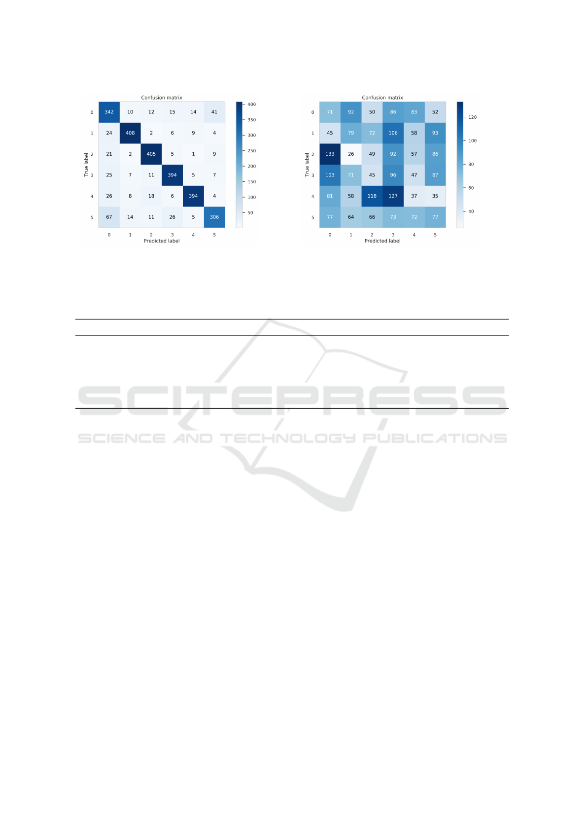
(a) Random Forest. (b) Agent TTR Prediction Performance per Class for Random

Forest (4a) and Random Guesser (4a) for the Customer Support

Topic Order.

Figure 4: Random Guesser Baseline.

Table 2: Agent Time-to-Reply (TTR) Results.

Topic Model Accuracy (std) AUC (std) F

-score (std) Hamming (std)

ChangeUser Random Forest 0.8720 (0.0214) 0.9232 (0.0128) 0.8720 (0.0214) 0.1279 (0.0214)

Baseline 0.1758 (0.0324) 0.5055 (0.0194) 0.1758 (0.0324) 0.8241 (0.0324)

Credit Random Forest 0.8149 (0.0096) 0.8889 (0.0057) 0.8149 (0.0096) 0.1850 (0.0096)

Baseline 0.1822 (0.0082) 0.5093 (0.0049) 0.1822 (0.0082) 0.8177 (0.0082)

Order Random Forest 0.8442 (0.0310) 0.9065 (0.0186) 0.8442 (0.0310) 0.1557 (0.0310)

Baseline 0.1535 (0.0114) 0.4921 (0.0068) 0.1535 (0.0114) 0.8464 (0.0114)

the models trained by the Random Forest algorithm

show interesting predictive results with an overall

AUC metric of 0.90, which signiﬁcantly outperforms

random chance.

Figure 4b shows the absolute confusion matrix

for the predicted agent response times vs. the true

agent response times for the Random Forest algo-

rithms (Figure 4a) and the Random Guesser baseline

(Figure 4). The matrix shows the aggregated results

over the different test folds showing that the Ran-

dom Guesser baseline classiﬁer randomly appoints

the classes. In contrast the Random Forest model has

a clear diagonal score that indicates signiﬁcantly bet-

ter prediction performance compared to the random

baseline.

This is supported by the results shown in Table 2

in which the Random Forest models have AUC scores

slightly above or below 0.9. In fact the 95 % con-

ﬁdence interval of the AUC metric for each of the

three class labels ChangeUser, Credit and Order were

0.92 ± 0.026, 0.89 ± 0.011 and 0.91 ± 0.037 respec-

tively. This indicates the the models have a good

ability to predict the TTR over various class labels.

This is further strengthened when evaluating the pre-

dictive performance in terms of accuracy or F

-scores

instead. Although using these metrics, the Random

Forest models still performs well above 0.80, whereas

the Random Guesser baseline models are associated

with useless scores at 0.18, or worse. Figure 4a fur-

ther indicates that the models have a slightly higher

misclassiﬁcation for label 0, and 5 compared to the

other labels. This indicate that TTR prediction within

2 hours and beyond 48 hours are slightly more difﬁ-

cult to predict.

5.2 Experiment 2: Customer Response

Prediction

Similar to the previous experiment, Figure 3 shows

that the Random Guesser baseline models have an

AUC metric of 0.50 while the Random Forest models

signiﬁcantly outperforms that with a metric of 0.85

when predicting customers’ e-mail response times.

Similar to the results in Section 5.1, Figure 5b shows

the absolute confusion matrix for the predicted agent

response times vs. the true agent response times for

the Random Forest models (Figure 5a) and the Ran-

dom Guesser baseline models (Figure 5).

The matrix shows the aggregated results over the

different test folds that clearly show the increased pre-

ICEIS 2020 - 22nd International Conference on Enterprise Information Systems

310

(a) Random Forest. (b) Customer TTR Prediction Performance per Class for

Random Forest (5a) and Random Guesser (5) for the Cus-

tomer Support Topic Order.

Figure 5: Random Guesser Classiﬁer.

Table 3: Customer Time-to-Reply (TTR) Results.

Topic Model Accuracy (std) AUC (std) F

-score (std) Hamming (std)

ChangeUser RF 0.7760 (0.0231) 0.8656 (0.0138) 0.7760 (0.0231) 0.2239 (0.0231)

Random 0.1592 (0.0223) 0.4955 (0.0134) 0.1592 (0.0223) 0.8407 (0.0223)

Credit RF 0.7486 (0.0088) 0.8491 (0.0053) 0.7486 (0.0088) 0.2513 (0.0088)

Random 0.1798 (0.0055) 0.5079 (0.0033) 0.1798 (0.0055) 0.8201 (0.0055)

Order RF 0.7640 (0.0154) 0.8584 (0.0092) 0.7640 (0.0154) 0.2359 (0.0154)

Random 0.1527 (0.0216) 0.4916 (0.0130) 0.1527 (0.0216) 0.8472 (0.0216)

dictability performance for the Random Forest mod-

els.

This is supported by the results shown in Ta-

ble 3 where the Random Forest models have F

-scores

around 0.75, whereas the Random Guesser baseline

have F

-scores around than 0.15. Further, the Ran-

dom Forest model have mean AUC scores between

0.85 and 0.87. In fact the 95 % conﬁdence interval

of the AUC metric for each of the three class labels

ChangeUser, Credit and Order were 0.87 ± 0.028,

0.85 ±0.011 and 0.86 ±0.018 respectively. Although

the metrics are slightly lower compared to the results

from the ﬁrst experiment, this similarly indicates the

potential in predicting TTR for e-mails.

Similar to Figure 4a, Figure 5a indicates that the

model have a higher misclassiﬁcation for label 0 and

5 than the other labels, indicating that a TTR within

2 hours and beyond 48 hours are more difﬁcult to

predict. Two things are different from Figure 4a.

First, label 3 is also more difﬁcult to predict. Sec-

ond, the misclassiﬁcations are slightly worse than for

Figure 4a.

6 ANALYSIS AND DISCUSSION

The results presented in Section 5 indicates that it

is possible to predict the response time for customer

support agents, as well as the response time for when

customers will respond to e-mails received. Orga-

nizations can beneﬁt from these conclusions in (at

least) two scenarios. First, by aggregating the cus-

tomer TTR, it is possible to more accurately predict

the workload of agents the next couple of days. This

can be useful for either increasing the workforce, or

shifting personnel working on other topics. Secondly,

given that a predicted customer TTR is low, it might

be advisable for support agents to focus on other e-

mails with a low predicted agent TTR while waiting,

in order to be able to respond quickly the customers

eventual reply.

Predicting the support agents TTR is also use-

ful since it can be used as a proxy to indicate the

emotional and cognitive load associated with each e-

mail (Rafaeli et al., 2019), enabling more experienced

agents to handle them, planning the agents’ workload

(e.g. several low agent TTR e-mails, or a few long

agent TTR e-mails). Further, predicting agent TTR

Predicting e-Mail Response Time in Corporate Customer Support

311

allow for customers to be alerted when a support er-

rand is predicted to take a longer time than usual.

Even though the feature set of this experiment is

based partly on related work and partly on domain

expertise, it is important to investigate that the mod-

els have not learnt trivial solutions. For this reason,

a random tree in the Random Forest model has been

extracted and visualized using the Graphviz frame-

work (Gansner and North, 2000), of which a sub-tree

can be seen in Figure 6. This tree indicates that the

model has indeed not learnt a trivial solution when

predicting TTR.

As a way to further investigate the internals of the

models trained by Random Forest, the ELI5 model in-

terpretation framework was used to estimate the fea-

tures’ impact on the model’s class assignment. Ta-

ble 4 shows the relative impact each feature has on

the predictive result in the Random Forest model. The

most highly ranked feature is Sender followed by the

Message length and Text complexity, which seem rea-

sonable.

Table 4: Feature Weights for a Model Predicting Customer

TTR.

Weight Feature

0.2988 ± 0.0899 Sender

0.2094 ± 0.0770 Message length

0.2092 ± 0.0772 Text complexity factor

0.1685 ± 0.0724 Text sentiment

0.0598 ± 0.0365 Old

0.0544 ± 0.0322 Customer escalated

0 ± 0.0000 Escalated

An example of an instance being predicted using a

Random Forest model can be seen in Figure 7, where

the probability and feature impact is shown for each

possible response time bin. This particular instance,

is a true positive as it is correctly assigned to the 4-8h

bin with an accuracy of 0.98 %. The most signiﬁ-

cant feature in favor for this decision is Sender that

is assigned a weight of +0.324. The feature BIAS is

the expected average score based on the distribution

of the data

. In this case, the BIAS is quite similar

between the classes as the data, after the preprocess-

ing, are balanced between the classes. Overall, this

analysis of feature impacts indicate that the model has

picked up patterns in the e-mails that are relevant for

predicting TTR. Thus, it can be concluded that the

models have not learned useless patterns from arte-

https://stackoverﬂow.com/questions/49402701/eli5-

explaining-prediction-xgboost-model, accessed: 2020-02-

facts in the data sets.

The results from both experiments in this study

suggests that the models’ performance are in line with

results from related research in the problem domain

of instant messaging: 0.71 accuracy (Pielot et al.,

2014), 0.89 accuracy (Huang and Ku, 2018), 0.90

accuracy (Avrahami and Hudson, 2006). These re-

sults compare well to the results in this study. See Ta-

ble 2 and Table 3 that have accuracy scores between

0.81 − 0.87 and 0.74 − 0.77 respectively. Thus, com-

pared to the state-of-the-art, the results presented in

this study indicates improved performance (AUC ≈

0.85, F

≈ 0.84, accuracy ≈ 0.82 in mean perfor-

mance for agent TTR), compared to the best perform-

ing model among related work that was ADABoost

(AUC = 0.72, F

= 0.45, accuracy = 0.46) (Yang

et al., 2017).

Finally, the problem was investigated separately

for support agents and for customers. The results sug-

gest that it is easier to predict the time to respond for

agents, than it is for customers (c.f. Figure 4a and Fig-

ure 5a). This supports the prior statement that in this

setting the agents can be considered a more homoge-

neous group due to similar training and experience,

whereas the customers could be regarded as a more

heterogeneous group of persons with different back-

ground and experiences.

7 CONCLUSION AND FUTURE

WORK

This study investigated the ability to predict e-mail

time-to-reply for both customer support agents as well

as customers in a customer support setting. The re-

sults indicate that it is possible to predict the time

agents will take to reply to an e-mail with an AUC of

0.90, using seven features extracted from the e-mails.

Further, that it is possible to predict the time-to-reply

for customers to respond with an AUC of 0.85. These

conclusions can be used to anticipate the staff needs

in customer support, but also indicate to customers

when an e-mail might take a longer time than ex-

pected to respond to. Additionally, given that time-

to-reply can be indicative of emotional and cognitive

load, it can also be used to better tailor message pri-

oritization, e.g. messages with a high cognitive load

might be more efﬁciently handled by senior customer

agents, and messages with a lower cognitive load by

junior customer agents.

As future work, it would be interesting to evaluate

this prediction in practice. Such an evaluation would

be two-fold. First, to what extent can this be used

to more effectively predict workload of the customer

ICEIS 2020 - 22nd International Conference on Enterprise Information Systems

312

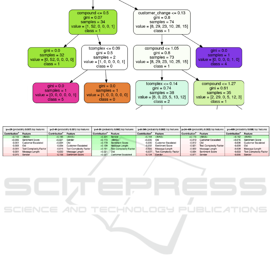
Figure 6: Sub-Tree Extracted from a Random Tree in a RF Model.

Figure 7: Prediction Explanation for a Random Instance in the Test Set for Customer TTR Prediction. The Instance Is a True

Positive, Where an Response Were Sent between 4-8 Hours from Receiving the E-Mail.

agents. Second, does it actually improve efﬁciency to

map cognitive and emotional load to different agents

based on experience.

REFERENCES

Abdallah, E., Abdallah, A. E., Bsoul, M., Otoom, A., and

Al Daoud, E. (2013). Simpliﬁed features for email

authorship identiﬁcation. International Journal of Se-

curity and Networks, 8:72–81.

Avrahami, D., Fussell, S. R., and Hudson, S. E. (2008).

Im waiting: Timing and responsiveness in semi-

synchronous communication. In Proceedings of the

2008 ACM Conference on Computer Supported Coop-

erative Work, CSCW ’08, pages 285–294, New York,

NY, USA. ACM.

Avrahami, D. and Hudson, S. E. (2006). Responsiveness

in instant messaging: Predictive models supporting

inter-personal communication. In Proceedings of the

SIGCHI Conference on Human Factors in Comput-

ing Systems, CHI ’06, pages 731–740, New York, NY,

USA. ACM.

Baron, N. S. (1998). Letters by phone or speech by other

means: the linguistics of email. Language & Commu-

nication, 18(2):133 – 170.

Batista, G. E., Bazzan, A. L., and Monard, M. C. (2003).

Balancing training data for automated annotation of

keywords: a case study. In WOB, pages 10–18.

Breiman, L. (2001). Random forests. Machine Learning,

45(1):5–32.

Church, K. and de Oliveira, R. (2013). What’s up with

whatsapp?: Comparing mobile instant messaging be-

haviors with traditional sms. In Proceedings of the

15th International Conference on Human-computer

Interaction with Mobile Devices and Services, Mo-

bileHCI ’13, pages 352–361, New York, NY, USA.

ACM.

Farr, J. N., Jenkins, J. J., and Paterson, D. G. (1951). Sim-

pliﬁcation of ﬂesch reading ease formula. Journal of

applied psychology, 35(5):333.

Fawcett, T. (2004). Roc graphs: Notes and practical consid-

erations for researchers. Machine learning, 31(1):1–

38.

Flach, P. (2012). Machine learning: the art and science of

algorithms that make sense of data. Cambridge Uni-

versity Press.

Gansner, E. R. and North, S. C. (2000). An open graph

visualization system and its applications to software

engineering. SOFTWARE - PRACTICE AND EXPE-

RIENCE, 30(11):1203–1233.

Halpin, N. (2016). The customer service report: Why great

customer service matters even more in the age of e-

commerce and the channels that perform best.

Huang, C. and Ku, L. (2018). Emotionpush: Emotion and

response time prediction towards human-like chat-

bots. In 2018 IEEE Global Communications Confer-

ence (GLOBECOM), pages 206–212.

Hutto, C. and Gilbert, E. (2015). Vader: A parsimonious

rule-based model for sentiment analysis of social me-

dia text.

Ikoro, G. O., Mondragon, R. J., and White, G. (2017). Pre-

Predicting e-Mail Response Time in Corporate Customer Support

313

dicting response waiting time in a chat room. In 2017

Computing Conference, pages 127–130.

Kooti, F., Aiello, L. M., Grbovic, M., Lerman, K., and

Mantrach, A. (2015). Evolution of conversations in

the age of email overload. In Proceedings of the 24th

International Conference on World Wide Web, WWW

’15, pages 603–613, Republic and Canton of Geneva,

Switzerland. International World Wide Web Confer-

ences Steering Committee.

Lema

ıtre, G., Nogueira, F., and Aridas, C. K. (2017).

Imbalanced-learn: A python toolbox to tackle the

curse of imbalanced datasets in machine learning.

Journal of Machine Learning Research, 18(17):1–5.

Pedregosa, F., Varoquaux, G., Gramfort, A., Michel, V.,

Thirion, B., Grisel, O., Blondel, M., Prettenhofer,

P., Weiss, R., Dubourg, V., Vanderplas, J., Passos,

A., Cournapeau, D., Brucher, M., Perrot, M., and

Duchesnay, E. (2011). Scikit-learn: Machine learning

in Python. Journal of Machine Learning Research,

12:2825–2830.

Pielot, M., de Oliveira, R., Kwak, H., and Oliver, N. (2014).

Didn’t you see my message?: Predicting attentiveness

to mobile instant messages. In Proceedings of the

32Nd Annual ACM Conference on Human Factors in

Computing Systems, CHI ’14, pages 3319–3328, New

York, NY, USA. ACM.

Rafaeli, A., Altman, D., and Yom-Tov, G. (2019). Cog-

nitive and emotional load inﬂuence response time of

service agents: A large scale analysis of chat service

conversations. In Proceedings of the 52nd Hawaii In-

ternational Conference on System Sciences.

Tsoumakas, G., Katakis, I., and Vlahavas, I. (2010). Min-

ing Multi-label Data, pages 667–685. Springer US,

Boston, MA.

Yang, L., Dumais, S. T., Bennett, P. N., and Awadallah,

A. H. (2017). Characterizing and predicting enterprise

email reply behavior. In Proceedings of the 40th Inter-

national ACM SIGIR Conference on Research and De-

velopment in Information Retrieval, SIGIR ’17, pages

235–244, New York, NY, USA. ACM.

Yang, Y. (1999). An evaluation of statistical approaches to

text categorization. Information Retrieval, 1(1):69–

90.

ICEIS 2020 - 22nd International Conference on Enterprise Information Systems

314