Learned and Hand-crafted Feature Fusion in Unit Ball for 3D Object

Classiﬁcation

Sameera Ramasinghe

1 a

, Salman Khan

2,1

and Nick Barnes

Australian National University, Australia

Inception Institute of Artiﬁcial Intelligence, U.A.E.

Keywords:

Convolution Neural Networks, Volumetric Convolution, Zernike Polynomials, Deep Learning.

Abstract:

Convolution is an effective technique that can be used to obtain abstract feature representations using hierarchical

layers in deep networks. However, performing convolution in non-Euclidean topological spaces such as the unit

ball (

) is still an under-explored problem. In this paper, we propose a light-weight experimental architecture

for 3D object classiﬁcation, that operates in

. The proposed network utilizes both hand-crafted and learned

features, and uses capsules in the penultimate layer to disentangle 3D shape features through pose and view

equivariance. It simultaneously maintains an intrinsic co-ordinate frame, where mutual relationships between

object parts are preserved. Furthermore, we show that the optimal view angles for extracting patterns from 3D

objects depend on its shape and achieve compelling results with a relatively shallow network, compared to the

state-of-the-art.

1 INTRODUCTION

Convolution is an extremely effective technique that

can be used to extract useful features from spatially

correlated data structures, with minimal supervision

((Krizhevsky et al., 2012; He et al., 2016)). Interest-

ingly, extending convolution to topological data struc-

tures other than Euclidean spaces, such as spheres,

is beneﬁcial to many research areas such as robotics,

geoscience and medical imaging, as real-world 3D

data naturally lie on a non-Euclidean manifold. The

aforementioned extension, however, is not straightfor-

ward due to the non-uniform grid structures of non-

Euclidean spaces, and is an open research problem.

Recently, there have been some key efforts to ex-

tend traditional convolution to spherical space. A pre-

liminary study of this was presented by (Boomsma

and Frellsen, 2017), where they apply a cube-sphere

transformation on 3D data, and add padding prior to

perform 2D convolution on the transformed data. The

work by (Cohen et al., 2018) recently received much at-

tention as they used spherical harmonics to efﬁciently

perform convolution on the surface of the sphere (

while achieving 3D rotational equivariance. A key

limitation of their work, however, is that the proposed

convolution operation is limited to polar shapes, as the

https://orcid.org/0000-0002-3200-9291

objects are represented in (

). In a slightly different

approach, (Weiler et al., 2018) proposed a method to

achieve SE(3) equivariance by modeling 3D data as

dense vector ﬁelds in 3D Euclidean space.

On the contrary, (Ramasinghe et al., 2019) pre-

sented a novel convolution operation that can perform

convolution in

. In this work, we adapt their derived

formulas and present a novel experimental architecture

which can be used to classify 3D objects. Our architec-

ture can handle non-polar shapes, and capture both 2D

texture and 3D shape features simultaneously. We use

a capsule network after the convolution layer as it al-

lows us to directly compare feature discriminability of

spherical convolution and volumetric convolution with-

out any bias. In other words, the optimum deep archi-

tecture for spherical convolution may not be the same

for volumetric convolution. Capsules, however, do not

deteriorate extracted features and the ﬁnal accuracy

only depends on the richness of input shape features.

Therefore, a fair comparison between spherical and

volumetric convolutions can be done by simply replac-

ing the convolution layer. Additionally, the proposed

architecture exploits both hand-crafted and learned fea-

tures and demonstrates that fusing these feature types

results in an improved performance. We show that the

optimum view-angles for extracting features from a 3D

object depends on its shape. We also demonstrate that

different learning models such as convolution and cap-

Ramasinghe, S., Khan, S. and Barnes, N.

Learned and Hand-crafted Feature Fusion in Unit Ball for 3D Object Classiﬁcation.

DOI: 10.5220/0009344801150125

In Proceedings of the 9th International Conference on Pattern Recognition Applications and Methods (ICPRAM 2020), pages 115-125

ISBN: 978-989-758-397-1; ISSN: 2184-4313

115

sule networks can work in unison towards a common

goal. Furthermore, our network achieves competitive

results with a signiﬁcantly shallow design, compared

to the state-of-the-art.

It is important to note that the proposed experimen-

tal architecture is only a one possible example out of

many possible designs, and is focused on three factors:

1) Capture useful features with a relatively shallow

network compared to state-of-the-art. 2) Show rich-

ness of computed features through clear improvements

over spherical convolution. 3) Demonstrate the useful-

ness of the volumetric convolution and axial symmetry

feature layers as fully differentiable and easily plug-

gable layers, which can be used as building blocks for

end-to-end deep architectures.

The rest of the paper is structured as follows. In

Sec. 2 we introduce the overall problem and our pro-

posed solution. Sec. 3 presents an overview of the

necessary theoretical background. Sec. 4.2 presents

our experimental architecture, and in Sec. 5 we show

the effectiveness of the derived operators through ex-

tensive experiments. Finally, we conclude the paper in

Sec. 6.

2 PROBLEM DEFINITION

Convolution is an effective method to capture useful

features from uniformly spaced grids in

, within

each dimension of

, such as gray scale images (

RGB images (

), spatio-temporal data (

) and

stacked planar feature maps (

). In such cases, uni-

formity of the grid within each dimension ensures the

translation equivariance of the convolution. However,

for topological spaces such as

and

, it is not pos-

sible to construct such a grid due to non-linearity. A

naive approach to perform convolution in

would

be to create a uniformly spaced three dimensional grid

(r,θ,φ)

coordinates (with necessary padding) and

perform 3D convolution. However, the spaces between

adjacent points in each axis are dependant on their ab-

solute position and hence, modeling such a space as a

uniformly spaced grid is not accurate.

To overcome these limitations, we propose a novel

experimental architecture which can effectively oper-

ate on functions in

. It is important to note that

ideally, the convolution in

should be a signal on

both 3D rotation group and 3D translation. However,

since Zernike polynomials do not have the necessary

properties to automatically achieve translation equiv-

ariance, we stick to 3D rotation group in this work.

In Sec. 3, we present an overview of the theoretical

background that is relevant to the context of this paper.

3 THEORETICAL BACKGROUND

3.1 3D Zernike Polynomials

3D Zernike polynomials are a complete and orthogo-

nal set of basis functions in

, that exhibits a ‘form

invariance’ property under 3D rotation ((Canterakis,

1999)). A

(n,l,m)

order 3D Zernike basis function

is deﬁned as,

n,l,m

= R

n,l

(r)Y

l,m

(θ,φ) (1)

where

n,l

is the Zernike radial polynomial,

l,m

(θ,φ)

is the spherical harmonics function,

n ∈ Z

l ∈ [0,n]

m ∈ [−l,l]

and

n − l

is even. Since 3D

Zernike polynomials are orthogonal and complete in

, an arbitrary function

f (r, θ,φ)

can be approx-

imated using Zernike polynomials as follows.

f (θ, φ,r) =

∞

∑

n=0

∑

l=0

∑

m=−l

Ω

n,l,m

( f )Z

n,l,m

(θ,φ, r) (2)

where Ω

n,l,m

( f ) could be obtained using,

Ω

n,l,m

( f ) =

2π

f (θ, φ,r)Z

†

n,l,m

sinφdrdφdθ

(3)

where

†

denotes the complex conjugate. In Sec. 3.2,

we will derive the proposed volumetric convolution.

3.2 Volumetric Convolution

Consider a 3D rotation operation, which moves a point

on the surface of the unit sphere to another point

. If we decompose the rotation using Eular angles

R(θ,φ) = R(θ)

R(φ)

R(θ)

, the ﬁrst rotation

R(θ)

can differ while mapping

(if

is the north pole).

In another words, there is no unique rotation operation

which can map

. However, enforcing the kernel

to be symmetric around the north pole (

-axis) makes

the rotated kernel function depend only on

and

since then the initial rotation around

does not affect

the kernel function. Following this observation, we are

able to deﬁne a 3D rotation kernel which only depends

on azimuth and polar angles, as shown in upcoming

derivations.

Let the kernel be symmetric around

and

f (θ, φ,r)

g(θ,φ, r)

be the functions of object and kernel respec-

tively. Then we deﬁne volumetric convolution as,

f ∗ g(α,β)

= h f (θ, φ,r), τ

(α,β)

(g(θ,φ,r))i

(4)

2π

f (θ,φ,r),τ

(α,β)

(g(θ,φ,r))sin φ dφdθdr,

(5)

ICPRAM 2020 - 9th International Conference on Pattern Recognition Applications and Methods

116

where

(α,β)

is an arbitrary rotation, that aligns the

north pole with the axis towards

(α,β)

direction (

and

are azimuth and polar angles respectively). Eq. 4

is able to capture more complex patterns compared

to spherical convolution due to two reasons: 1) the

inner product integrates along the radius and 2) the

projection onto spherical harmonics forces the function

into a polar function, that can result in information

loss.

(Ramasinghe et al., 2019) present the following

theorem to present volumetric convolution. A short

version of the proof is then provided. Please see Ap-

pendix 6 for the complete derivation.

Theorem 1:

Suppose

f ,g : X −→ R

are square

integrable complex functions deﬁned in

so that

h f , f i < ∞

and

hg,gi < ∞

. Further, suppose

is sym-

metric around north pole and

τ(α,β) = R

(α)R

(β)

where R ∈ SO(3). Then,

2π

f (θ, φ,r),τ

(α,β)

(g(θ,φ, r)) sinφ dφdθdr

≡

4π

∞

∑

n=0

∑

l=0

∑

m=−l

Ω

n,l,m

( f )Ω

n,l,0

(g)Y

l,m

(α,β),

(6)

where

Ω

n,l,m

( f ),Ω

n,l,0

(g)

and

l,m

(θ,φ)

are

(n,l,m)

3D Zernike moment of

(n,l,0)

3D Zernike moment

of g, and spherical harmonics function respectively.

Proof:

Completeness property of 3D Zernike Poly-

nomials ensures that it can approximate an arbitrary

function in

, as shown in Eq. 2. Leveraging this

property, Eq. 4 can be rewritten as,

f ∗ g(α,β) = h

∞

∑

n=0

∑

l=0

∑

m=−l

Ω

n,l,m

( f )Z

n,l,m

(α,β)

(

∞

∑

=−l

Ω

(g)Z

)i.

(7)

However, since

g(θ,φ, r)

is symmetric around

the rotation around

should not change the function.

This ensures,

g(r,θ, φ) = g(r,θ − α,φ) (8)

and hence,

∞

∑

=−l

Ω

(g)R

(r)Y

(θ,φ)

∞

∑

=−l

Ω

(g)R

(r)Y

(θ,φ)e

−im

(9)

This is true, if and only if

= 0

. Therefore, a symmet-

ric function around

, deﬁned inside the unit sphere

can be rewritten as,

∞

∑

Ω

(g)Z

(10)

which simpliﬁes Eq. 7 to,

f ∗ g(α,β) = h

∞

∑

n=0

∑

l=0

∑

m=−l

Ω

n,l,m

( f )Z

n,l,m

(α,β)

(

∞

∑

Ω

(g)Z

(11)

Using the properties of inner product, Eq. 11 can be

rearranged as,

f ∗ g(α,β) =

∞

∑

n=0

∑

l=0

∞

∑

m=−l

Ω

n,l,m

( f )Ω

(g)

n,l,m

,τ

(α,β)

)i. (12)

Using the rotational properties of Zernike polynomials,

we obtain (see Appendix 6 for our full derivation),

f ∗ g(θ,φ) =

4π

∞

∑

n=0

∑

l=0

∑

m=−l

Ω

n,l,m

( f )Ω

n,l,0

(g)Y

l,m

(θ,φ)

(13)

Since we can calculate

Ω

n,l,m

( f )

and

Ω

n,l,0

(g)

eas-

ily using an iterative method ((Ramasinghe et al.,

2019)),

f ∗ g(θ,φ)

can be found using a simple ma-

trix multiplication. It is interesting to note that,

since the convolution kernel does not translate, the

convolution produces a polar shape, which can be

further convolved–if needed–using the relationship

f ∗ g(θ,φ) =

4π

2l+1

∑

m=−l

f (l,m) ˆg(l, m)Y

(l,m)

(θ,φ)

where,

f (l,m)

and

ˆg(l, m)

are the

(l, m)

frequency

components of f and g in spherical harmonics space.

3.3 Equivariance to 3D Rotation Group

The equivariance of the volumetric convolution to 3D

rotation group can be shown using the following theo-

rem.

Theorem 1:

Suppose

f ,g : X −→ R

are square

integrable complex functions deﬁned in

so that

h f , f i < ∞

and

hg,gi < ∞

. Also, let

α,β,γ

be a

3D rotation operator that can be decomposed into

three Eular rotations

(α)R

(β)R

(γ)

and

α,β

an-

other rotation operator that can be decomposed into

(α)R

(β)

. Suppose

α,β,γ

(g) = τ

α,β

(g)

. Then,

(α,β,γ)

( f ) ∗ g(θ,φ) = τ

(α,β)

( f ∗ g)(θ,φ)

, where

∗

the volumetric convolution operator.

The proof to above theorem can be found in Ap-

pendix 6.

Learned and Hand-crafted Feature Fusion in Unit Ball for 3D Object Classiﬁcation

117

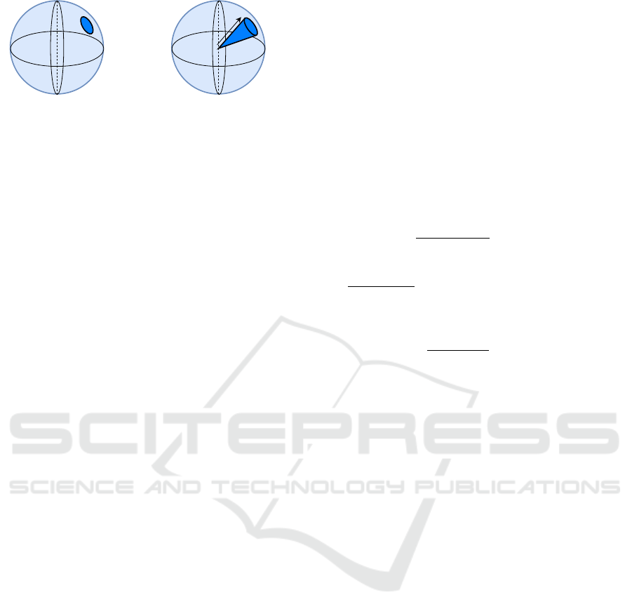
(θ ,ϕ )(θ ,ϕ )

Figure 1: Difference between spherical convolution (left) and

volumetric convolution (right). In volumetric convolution,

inner product between kernel and the shape is taken in

and in spherical convolution, it is taken in

. Modeling and

convolving in

allows encoding non-polar 3D shapes with

texture.

3.4 Axial Symmetry of Functions in B

Axial symmetry of a function in

around an arbitrary

axis can be found using the following formula.

Proposition:

Suppose

g : X −→ R

is a square

integrable complex function deﬁned in

such that

hg,gi < ∞

. Then, the power of projection of

in to

S =

}

where

is the set of Zernike basis functions that

are symmetric around an axis towards

(α,β)

direction

is given by,

||sym

(α,β)

||=

∑

l=0

∑

m=−l

Ω

n,l,m

m,l

(α,β)||

(14)

where

and

are azimuth and polar angles respec-

tively.

The proof the above proposition is given in Ap-

pendix 6.

4 A CASE STUDY: 3D OBJECT

RECOGNITION

4.1 3D Objects as Functions in B

A polar 3D object can be expressed as a single val-

ued function on the

. Performing convolution on

can be considered as moving the kernel on

and

then calculating inner product with the shape func-

tion. However, representing non-polar shapes as polar

objects can lead to critical information loss. Further-

more, since the inner produce happens on

, it is not

possible to capture patterns across radius.

The aforementioned limitations can be avoided

by performing convolution inside the unit ball (

Modeling the shape functions inside

allows us to

represent non-polar shapes without loss of informa-

tion and it allows encoding 2D texture information, as

each point inside

can be allocated a scalar value.

Figure 1 illustrates the difference between volumetric

and spherical convolutions. However, we experiment

only on uniform textured 3D objects in this work, and

therefore, apply an artiﬁcial surface function to the

objects as follows:

f (θ, φ,r) =

(

r, if surface exists at (θ,φ, r)

0, otherwise

(15)

4.2 An Experimental Architecture

We implement an experimental architecture to demon-

strate the usefulness of the proposed operations. While

these operations can be used as building-tools to con-

struct any deep network, we focus on three key fac-

tors while developing the presented experimental ar-

chitecture: 1)

Shallowness:

Volumetric convolution

should be able to capture useful features compared

to other methodologies with less number of layers.

Modularity:

The architecture should have a mod-

ular nature so that a fair comparison can be made

between volumetric and spherical convolution. We

use a capsule network after the convolution layer for

this purpose. 3)

Flexibility:

It should clearly exhibit

the usefulness of axial symmetry features as a hand-

crafted and fully differentiable layer. The motivation

is to demonstrate one possible use case of axial sym-

metry measurements in 3D shape analysis.

The proposed architecture consists of four compo-

nents.

First

, we obtain three view angles, and later

generate features for each view angle separately. We

optimize the view angles to capture complimentary

shape details such that the total information content is

maximized. For each viewing angle ‘

’, we obtain two

point sets P

and P

−

consisting of tuples denoted as:

= {(x

) : y

> 0}, and

−

= {(x

) : y

< 0}, (16)

such that

denotes the horizontal axis.

Second

, the six

point sets are volumetrically convolved with kernels

to capture local patterns of the object. The generated

features for each point set are then combined using

compact bilinear pooling.

Third

, we use axial sym-

metry measurements to generate additional features.

The features that represent each point set are then com-

bined using compact bilinear pooling.

Fourth

, we

feed features from second and third components of

the overall architecture to two independent capsule

networks and combine the outputs at decision level to

obtain the ﬁnal prediction. The overall architecture of

the proposed scheme is shown in Fig. 2.

4.3 Optimum View Angles

We use three view angles to generate features for bet-

ter representation of the object. First, we translate

ICPRAM 2020 - 9th International Conference on Pattern Recognition Applications and Methods

118

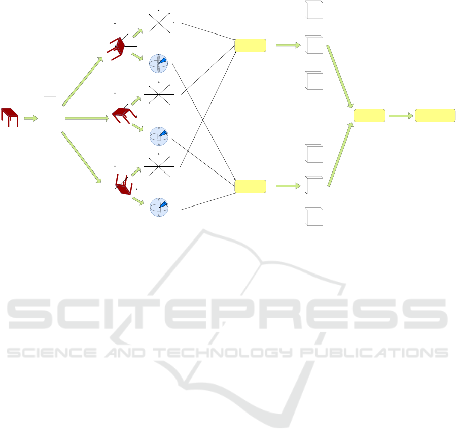
CBP

Max-Pool

Classiﬁcation

1-D ConvNet

Figure 2: Experimental architecture: An object is ﬁrst mapped to three view angles. For each angle, axial symmetry and

volumetric convolution features are generated for

and

−

. These two features are then separately combined using compact

bilinear pooling. Finally, the features are fed to two individual capsule networks, and the decisions are max-pooled.

the center of mass of the set of

(x,y, z)

points to the

origin. The goal of this step is to achieve a general

translational invariance, which allows us to free the

convolution operation from the burden of detecting

translated local patterns. Subsequently, the point set is

rearranged as an ordered set on

and

and a 1D convo-

lution net is applied on

values of the points. Here, the

objective is to capture local variations of points along

the

axis, since later we analyze point sets

and

−

independently. The trained ﬁlters can be assumed

to capture properties similar to

∂

y/∂x

and

∂

y/∂z

where

is the order of derivative. The output of the 1D

convolution net is rotation parameters represented by a

1 × 9

vector

~r = {r

,· ·· ,r

}

. Then, we compute

= R

)

= R

)

and

= R

)

where

and

are

the rotations that map the points to three different view

angles.

After mapping the original point set to three view

angles, we extract the

and

−

point sets from each

angle

that gives us six point sets. These sets are

then fed to the volumetric convolution layer to obtain

feature maps for each point set. We then measure the

symmetry around four equi-angular axes using Eq. 14,

and concatenate these measurement values to form a

feature vector for the same point sets.

4.4 Feature Fusion using Compact

Bilinear Pooling

Compact bilinear pooling (CBP) provides a compact

representation of the full bilinear representation, but

has the same discriminative power. The key advantage

of compact bilinear pooling is the signiﬁcantly reduced

dimensionality of the pooled feature vector.

We ﬁrst concatenate the obtained volumetric con-

volution features of the three angles, for

and

−

separately to establish two feature vectors. These two

features are then fused using compact bilinear pooling

((Gao et al., 2016)). The same approach is used to

combine the axial symmetry features. These fused

vectors are fed to two independent capsule nets.

Furthermore, we experiment with several other fea-

ture fusion techniques and present results in Sec. 5.2.

4.5 Capsule Network

Capsule Network (CapsNet) ((Sabour et al., 2017))

brings a new paradigm to deep learning by modeling

input domain variations through vector based repre-

sentations. CapsNets are inspired by so-called inverse

graphics, i.e., the opposite operation of image render-

ing. Given a feature representation, CapsNets attempt

to generate the corresponding geometrical representa-

tion. The motivation for using CapsNets in the network

are twofold: 1) CapsNet promotes a dynamic ‘routing-

by-agreement’ approach where only the features that

Learned and Hand-crafted Feature Fusion in Unit Ball for 3D Object Classiﬁcation

119

are in agreement with high-level detectors are routed

forward. This property of CapsNets does not deteri-

orate extracted features and the ﬁnal accuracy only

depends on the richness of original shape features. It

allows us to directly compare feature discriminability

of spherical and volumetric convolution without any

bias. For example, using multiple layers of volumetric

or spherical convolution hampers a fair comparison

since it can be argued that the optimum architecture

may vary for two different operations. 2) CapsNet pro-

vides an ideal mechanism for disentangling 3D shape

features through pose and view equivariance while

maintaining an intrinsic co-ordinate frame where mu-

tual relationships between object parts are preserved.

Inspired by these intuitions, we employ two in-

dependent CapsNets in our network for volumetric

convolution features and axial symmetry features. In

this layer, we rearrange the input feature vectors as

two sets of primary capsules—for each capsule net—

and use the dynamic routing technique proposed by

(Sabour et al., 2017) to predict the classiﬁcation results.

The outputs are then combined using max-pooling, to

obtain the ﬁnal classiﬁcation result. For volumetric

convolution features, our architecture uses

1000

pri-

mary capsules with

dimensions each. For axial

symmetry features, we use

2500

capsules, each with

dimensions. In both networks, decision layer con-

sist of 12 dimensional capsules.

4.6 Hyperparameters

We use

n = 5

to implement Eq. 13 and use a decaying

learning rate

lr = 0.1 × 0.9

step

3000

, where

step

is incre-

mented by one per each iteration. For training, we use

the Adam optimizer with

= 0.9, β

= 0.999, ε =

1 × 10

−8

where parameters refer to the usual notation.

All these values are chosen empirically. Since we have

decomposed the theoretical derivations into sets of

low-cost matrix multiplications, speciﬁcally aiming to

reduce the computational complexity, the GPU imple-

mentation is highly efﬁcient. For example, the model

takes less than 15 minutes for an epoch during the

training phase for ModelNet10, with a batchsize 2, on

a single GTX 1080Ti GPU.

5 EXPERIMENTS

In this section, we discuss and evaluate the perfor-

mance of the proposed approach. We ﬁrst compare the

accuracy of our model with relevant state-of-the-art

work, and then present a thorough ablation study of

our model, that highlights the importance of several

architectural aspects. We use ModelNet10 and Model-

Net40 datasets in our experiments. Next, we evaluate

the robustness of our approach against loss of informa-

tion and ﬁnally show that the proposed approach for

computing 3D Zernike moments produce richer repre-

sentations of 3D shapes, compared to the conventional

approach.

5.1 Comparison with the

State-of-the-art

Table 1 illustrates the performance comparison of our

model with state-of-the-art. The model attains an over-

all accuracy of

92.17%

on ModelNet10 and

86.5%

accuracy on ModelNet40, which is on par with state-

of-the-art. We do not compare with other recent work,

such as (Kanezaki et al., 2016), (Qi et al., 2016),

(Sedaghat et al., 2016), (Wu et al., 2016), (Qi et al.,

2016) and (Bai et al., 2016), (Maturana and Scherer,

2015) that show impressive performance on Model-

Net10 and ModelNet40. These are not comparable

with our proposed approach, as we propose a shallow,

single model without any data augmentation, with a

relatively low number of parameters. Furthermore,

our model reports these results by using only a sin-

gle volumetric convolution layer for learning features.

Fig. 3 demonstrates effectiveness of our architecture

by comparing accuracy against the number of trainable

parameters in state-of-the-art models.

5.2 Ablation Study

Table 2 depicts the performance comparison between

several variants of our model. To highlight the ef-

fectiveness of the learned optimum view points, we

replace the optimum view point layer with three ﬁxed

orthogonal view points. This modiﬁcation causes an

accuracy drop of 6.57%, emphasizing that the opti-

mum view points indeed depends on the shape. An-

other interesting—perhaps the most important—aspect

to study is the performance of the proposed volumet-

ric convolution against spherical convolution. To this

end, we replace the volumetric convolution layer of

our model with spherical convolution and compare

the results. It can be seen that our volumetric convo-

lution scheme outperforms spherical convolution by

a signiﬁcant margin of 12.56%, indicating that vol-

umetric convolution captures shape properties more

effectively.

Furthermore, using mean-pooling instead of max-

pooling, at the decision layer drops the accuracy to

87.27%

. We also evaluate performance of using a sin-

gle capsule net. In this scenario, we combine axial

symmetry features with volumetric convolution fea-

ICPRAM 2020 - 9th International Conference on Pattern Recognition Applications and Methods

120

Table 1: Comparison with state-of-the-art methods on ModelNet10 and ModelNet40 datasets (ranked according to performance).

Ours achieve a competitive performance with the least network depth.

Method Trainable layers # Params M10 M40

SO-Net ((Li et al., 2018)) 11FC 60M 95.7% 93.4%

Kd-Networks ((Klokov and Lempitsky, 2017)) 15KD - 94.0% 91.8%

VRN ((Brock et al., 2016)) 45Conv 90M 93.11% 90.8%

Pairwise ((Johns et al., 2016)) 23Conv 143M 92.8% 90.7%

MVCNN ((Su et al., 2015)) 60Conv + 36FC 200M - 90.1%

Ours 3Conv + 2Caps 4.4M 92.17% 86.5%

PointNet ((Qi et al., 2017)) 2ST + 5Conv 80M - 86.2%

ECC ((Simonovsky and Komodakis, 2017)) 4Conv + 1FC - - 83.2%

DeepPano ((Shi et al., 2015)) 4Conv + 3FC - 85.45% 77,63%

3DShapeNets ((Wu et al., 2015)) 4-3DConv + 2FC 38M 83.5% 77%

PointNet ((Garcia-Garcia et al., 2016)) 2Conv + 2FC 80M 77.6% -

Table 2: Ablation study of the proposed architecture on

ModelNet10 dataset.

Method Accuracy

Final Architecture (FA) 92.17%

FA + Orthogonal Rotation 85.60%

FA - VolCNN + SphCNN 79.53%

FA -MaxPool + MeanPool 87.27%

FA + Feature Fusion (Axial + Conv) 86.53%

Axial Symmetry Features 66.73%

VolConv Features 85.3%

SphConv Features 71.6%

FA - CapsNet + FC layers 87.3 %

FA - CBP + Feature concat 90.7%

FA - CBP + MaxPool 90.3%

FA - CBP + Average-pooling 85.3 %

20 40 60 80 100 120 140 160 180 200

100

SO-Net

VRN

Pairwise

MVCNN

Ours

PointNet

3DShapeNet

Accuracy

Number of trainable parameters

Figure 3: Accuracy vs number of trainable params (in mil-

lions) trend (ModelNet40).

tures using compact bilinear pooling (CBP), and feed

it a single capsule network. This variant achieves an

overall accuracy of

86.53%

, is a

5.64%

reduction in

accuracy compared to the model with two capsule net-

works.

Moreover, we compare the performance of two

feature categories—volumetric convolution features

and axial symmetry features—individually. Axial sym-

metry features alone are able to obtain an accuracy of

66.73%

, while volumetric convolution features reach a

signiﬁcant

85.3%

accuracy. On the contrary, spherical

convolution attains an accuracy of

71.6%

, which again

highlights the effectiveness of volumetric convolution.

Then we compare between different choices that

can be applied to the experimental architecture. We

ﬁrst replace the capsule network with a fully connected

layer and achieve an accuracy of 87.3%. This is per-

haps because capsules are superior to a simple fully

connected layer in modeling view-point invariant rep-

resentations. Then we try different substitutions for

compact bilinear pooling and achieve 90.7%, 90.3%

and 85.3% accuracies respectively for feature concate-

nation, max-pooling and average-pooling. This justi-

ﬁes the choice of compact bilinear pooling as a feature

fusion tool. However, it should be noted that these

choices may differ depending on the architecture.

5.3 Rotation Parameters

The optimum view-angles for learning features in 3D

space depend on the geometric features of a particular

3D object. Therefore, allowing the network to learn

these optimum view-angles, in contrast to using ﬁxed

angles for every shape, improves the performance, as

discussed in Section 5.2. Table 3 depicts the ﬁnal

rotation parameters learned by the network, which

are then used for rotating the object. As it is clearly

evident, each shape category corresponds to different

rotation parameters, which empirically proves that the

optimum view-angles indeed depend on the object

class.

Learned and Hand-crafted Feature Fusion in Unit Ball for 3D Object Classiﬁcation

121

Table 3: Average rotation parameter values across classes of ModelNet10. The values are reformatted to be positive angles

between 0 and 360.

Class r

Bathtub Bathtub 319.2 100.5 57.8 185.2 223.4 98.3 350.6 167.4 14.2

Bed 264.3 196.3 103.7 208.5 186.2 194.4 267.9 246.3 81.2

Chair 198.6 91.2 243.7 47.4 161.2 87.9 240.5 47.3 203.4

Desk 88.4 80.2 130.9 206.6 86.5 112.8 291.7 233.2 351.4

Dresser 58.0 145.7 353.1 148.4 346.4 125.3 47.0 2.2 35.4

Monitor 218.9 279.0 58.1 10.4 30.3 331.4 90.7 285.6 346.1

Night stand 85.3 336.1 175.9 246.4 169.4 278.7 317.0 137.6 302.9

Sofa 306.1 86.9 109.2 311.1 22.5 321.4 96.9 47.0 76.2

Table 299.8 85.2 126.5 215.1 221.9 245.5 237.1 50.6 128.4

Toilet 277.0 325.3 215.5 255.6 192.2 19.8 278.4 193.4 348.2

Average 211.6 172.6 157.4 183.4 164.1 182.4 221.8 141.1 189.7

6 CONCLUSION

In this work, we present a novel experimental archi-

tecture, which can learn feature representations in

We utilize the underlying theoretical foundations for

volumetric convolution and demonstrate how it can

be efﬁciently computed and implemented using low-

cost matrix multiplications. Moreover, we show that

our experimental architecture gives competitive results

to state-of-the-art with a relatively shallow design, in

3D object recognition task. Finally, we empirically

demonstrate that fusing learned and hand-crafted fea-

tures results in improved performance, as they provide

complementary information.

REFERENCES

Bai, S., Bai, X., Zhou, Z., Zhang, Z., and Latecki, L. J.

(2016). Gift: A real-time and scalable 3d shape search

engine. In Computer Vision and Pattern Recognition

(CVPR), 2016 IEEE Conference on, pages 5023–5032.

IEEE.

Boomsma, W. and Frellsen, J. (2017). Spherical convolu-

tions and their application in molecular modelling. In

Advances in Neural Information Processing Systems,

pages 3436–3446.

Brock, A., Lim, T., Ritchie, J. M., and Weston, N.

(2016). Generative and discriminative voxel modeling

with convolutional neural networks. arXiv preprint

arXiv:1608.04236.

Canterakis, N. (1999). 3d zernike moments and zernike

afﬁne invariants for 3d image analysis and recogni-

tion. In In 11th Scandinavian Conf. on Image Analysis.

Citeseer.

Cohen, T. S., Geiger, M., Koehler, J., and Welling, M. (2018).

Spherical cnns. International Conference on Learning

representations (ICLR).

Gao, Y., Beijbom, O., Zhang, N., and Darrell, T. (2016).

Compact bilinear pooling. In Proceedings of the IEEE

Conference on Computer Vision and Pattern Recogni-

tion, pages 317–326.

Garcia-Garcia, A., Gomez-Donoso, F., Garcia-Rodriguez, J.,

Orts-Escolano, S., Cazorla, M., and Azorin-Lopez, J.

(2016). Pointnet: A 3d convolutional neural network

for real-time object class recognition. In Neural Net-

works (IJCNN), 2016 International Joint Conference

on, pages 1578–1584. IEEE.

He, K., Zhang, X., Ren, S., and Sun, J. (2016). Deep resid-

ual learning for image recognition. In Proceedings of

the IEEE conference on computer vision and pattern

recognition, pages 770–778.

Johns, E., Leutenegger, S., and Davison, A. J. (2016). Pair-

wise decomposition of image sequences for active

multi-view recognition. In Computer Vision and Pat-

tern Recognition (CVPR), 2016 IEEE Conference on,

pages 3813–3822. IEEE.

Kanezaki, A., Matsushita, Y., and Nishida, Y. (2016). Rota-

tionnet: Joint object categorization and pose estimation

using multiviews from unsupervised viewpoints. arXiv

preprint arXiv:1603.06208.

Klokov, R. and Lempitsky, V. (2017). Escape from cells:

Deep kd-networks for the recognition of 3d point cloud

models. In 2017 IEEE International Conference on

Computer Vision (ICCV), pages 863–872. IEEE.

Krizhevsky, A., Sutskever, I., and Hinton, G. E. (2012). Im-

agenet classiﬁcation with deep convolutional neural

networks. In Advances in neural information process-

ing systems, pages 1097–1105.

Li, J., Chen, B. M., and Lee, G. H. (2018). So-net: Self-

organizing network for point cloud analysis. arXiv

preprint arXiv:1803.04249.

Maturana, D. and Scherer, S. (2015). Voxnet: A 3d convo-

lutional neural network for real-time object recogni-

tion. In Intelligent Robots and Systems (IROS), 2015

IEEE/RSJ International Conference on, pages 922–928.

IEEE.

Qi, C. R., Su, H., Mo, K., and Guibas, L. J. (2017). Point-

ICPRAM 2020 - 9th International Conference on Pattern Recognition Applications and Methods

122

net: Deep learning on point sets for 3d classiﬁcation

and segmentation. Proc. Computer Vision and Pattern

Recognition (CVPR), IEEE, 1(2):4.

Qi, C. R., Su, H., Nießner, M., Dai, A., Yan, M., and Guibas,

L. J. (2016). Volumetric and multi-view cnns for object

classiﬁcation on 3d data. In Proceedings of the IEEE

conference on computer vision and pattern recognition,

pages 5648–5656.

Ramasinghe, S., Khan, S., Barnes, N., and Gould, S.

(2019). Representation learning on unit ball with

3d roto-translational equivariance. arXiv preprint

arXiv:1912.01454.

Sabour, S., Frosst, N., and Hinton, G. E. (2017). Dynamic

routing between capsules. In Advances in Neural In-

formation Processing Systems, pages 3859–3869.

Sedaghat, N., Zolfaghari, M., Amiri, E., and Brox, T. (2016).

Orientation-boosted voxel nets for 3d object recogni-

tion. arXiv preprint arXiv:1604.03351.

Shi, B., Bai, S., Zhou, Z., and Bai, X. (2015). Deeppano:

Deep panoramic representation for 3-d shape recog-

nition. IEEE Signal Processing Letters, 22(12):2339–

2343.

Simonovsky, M. and Komodakis, N. (2017). Dynamic edge-

conditioned ﬁlters in convolutional neural networks on

graphs. In Proc. CVPR.

Su, H., Maji, S., Kalogerakis, E., and Learned-Miller, E.

(2015). Multi-view convolutional neural networks for

3d shape recognition. In Proceedings of the IEEE

international conference on computer vision, pages

945–953.

Weiler, M., Geiger, M., Welling, M., Boomsma, W., and Co-

hen, T. (2018). 3d steerable cnns: Learning rotationally

equivariant features in volumetric data. arXiv preprint

arXiv:1807.02547.

Wu, J., Zhang, C., Xue, T., Freeman, B., and Tenenbaum,

J. (2016). Learning a probabilistic latent space of ob-

ject shapes via 3d generative-adversarial modeling. In

Advances in Neural Information Processing Systems,

pages 82–90.

Wu, Z., Song, S., Khosla, A., Yu, F., Zhang, L., Tang, X., and

Xiao, J. (2015). 3d shapenets: A deep representation

for volumetric shapes. In Proceedings of the IEEE

conference on computer vision and pattern recognition,

pages 1912–1920.

APPENDIX

Convolution within Unit Sphere using 3D

Zernike Polynomials

Theorem 1:

Suppose

f ,g : X −→ R

are square

integrable complex functions deﬁned in

so that

h f , f i < ∞

and

hg,gi < ∞

. Further, suppose

is sym-

metric around north pole and

τ(α,β) = R

(α)R

(β)

where R ∈ SO(3). Then,

2π

f (θ, φ,r),τ

(α,β)

(g(θ,φ, r)) sinφ dφdθdr

≡

4π

∞

∑

n=0

∑

l=0

∑

m=−l

Ω

n,l,m

( f )Ω

n,l,0

(g)Y

l,m

(α,β),

(17)

where

Ω

n,l,m

( f ),Ω

n,l,0

(g)

and

l,m

(θ,φ)

are

(n,l,m)

3D Zernike moment of

(n,l,0)

3D Zernike moment

of g, and spherical harmonics function respectively.

Proof:

Since 3D Zernike polynomials are orthog-

onal and complete in

, an arbitrary function

f (r, θ,φ)

can be approximated using Zernike polynomials

as follows.

f (θ, φ,r) =

∞

∑

n=0

∑

l=0

∑

m=−l

Ω

n,l,m

( f )Z

n,l,m

(θ,φ, r) (18)

where Ω

n,l,m

( f ) could be obtained using,

Ω

n,l,m

( f ) =

2π

f (θ, φ,r)Z

†

n,l,m

sinφdrdφdθ

(19)

where

†

denotes the complex conjugate.

Leveraging this property (Eq. 18) of 3D Zernike

polynomials Eq. 4 can be rewritten as,

f ∗ g(α,β) = h

∞

∑

n=0

∑

l=0

∑

m=−l

Ω

n,l,m

( f )Z

n,l,m

(α,β)

(

∞

∑

=−l

Ω

(g)Z

)i.

(20)

But since

g(θ,φ, r)

is symmetric around

, the rota-

tion around

should not change the function. Which

ensures,

g(r,θ, φ) = g(r,θ − α,φ) (21)

and hence,

∞

∑

=−l

Ω

(g)R

(r)Y

(θ,φ)

∞

∑

=−l

Ω

(g)R

(r)Y

(θ,φ)e

−im

(22)

This is true, if and only if

= 0

. Therefore, a

symmetric function around

, deﬁned inside the unit

sphere can be rewritten as,

∞

∑

Ω

(g)Z

(23)

Learned and Hand-crafted Feature Fusion in Unit Ball for 3D Object Classiﬁcation

123

which simpliﬁes Eq. 20 to,

f ∗ g(α,β) = h

∞

∑

n=0

∑

l=0

∑

m=−l

Ω

n,l,m

( f )Z

n,l,m

(α,β)

(

∞

∑

Ω

(g)Z

(24)

Using the properties of inner product, Eq. 24 can

be rearranged as,

f ∗ g(α,β) =

∞

∑

n=0

∑

l=0

∞

∑

m=−l

Ω

n,l,m

( f )Ω

(g)

n,l,m

,τ

(α,β)

)i. (25)

Consider the term τ

(α,β)

). Then,

(α,β)

(θ,φ,r)) = τ

(α,β)

(r)Y

(θ,φ))

= R

(r)τ

(α,β)

(θ,φ))

= R

(r)

∑

=−l

(θ,φ)D

(α,β,·),

(26)

where

m,m

is the Wigner-D matrix. But we know

that D

(θ,φ) = Y

(θ,φ). Then Eq. 25 becomes,

f ∗ g(α,β) =

∞

∑

n=0

∑

l=0

∞

∑

m=−l

Ω

n,l,m

( f )Ω

(g)

∑

=−l

(α,β)hZ

n,l,m

i, (27)

f ∗ g(α,β) =

4π

∞

∑

n=0

∑

l=0

∑

m=−l

Ω

n,l,m

( f )Ω

n,l,0

(g)Y

l,m

(α,β),

(28)

Equivariance of Volumetric Convolution

to 3D Rotation Group

Theorem 2:

Suppose

f ,g : B

−→ R

are square in-

tegrable complex functions deﬁned in

such that

h f , f i < ∞

and

hg,gi < ∞

. Also, let

α,β,γ

be a 3D rota-

tion operator that can be decomposed into three Euler

rotations

(α)R

(β)R

(γ)

and

α,β

another rotation

operator that can be decomposed into

(α)R

(β)

Suppose η

α,β,γ

(g) = τ

α,β

(g). Then,

(α,β,γ)

( f ) ∗ g(θ,φ) = τ

(α,β)

( f ∗ g)(θ, φ), (29)

where ∗ is the volumetric convolution operator.

Proof:

Since

(α,β,γ)

∈ SO(3)

, we know that

(α,β,γ)

( f (x)) = f (η

−1

(α,β,γ)

(x))

. Also we know that

(α,β,γ)

: R

→ R

is an isometry. We deﬁne,

hη

(α,β,γ)

f ,η

(α,β,γ)

gi =

f (η

−1

(α,β,γ)

(x))g(η

−1

(α,β,γ)

(x))dx.

(30)

Consider the Lebesgue measure

λ(B

) =

. It

can be proven that a Lebesgue measure is invariant un-

der the isometries, which gives us

dx = dη

(α,β,γ)

(x) =

dη

−1

(α,β,γ)

(x),∀x ∈ B

. Therefore,

hη

(α,β,γ)

f ,η

(α,β,γ)

gi = h f , gi

f (η

−1

(α,β,γ)

(x))g(η

−1

(α,β,γ)

(x))d(η

−1

(α,β,γ)

x).

(31)

Let

f (θ, φ,r)

and

g(θ,φ, r)

be the object function

and kernel function (symmetric around north pole)

respectively. Then volumetric convolution is deﬁned

f ∗ g(θ,φ) = h f , τ

(θ,φ)

gi. (32)

Applying the rotation η

(α,β,γ)

to f , we get

(α,β,γ)

( f ) ∗ g(θ,φ) = hη

(α,β,γ)

( f ),τ

(θ,φ)

gi (33)

Using the result in Eq. 31, we have

(α,β,γ)

( f ) ∗ g(θ,φ) = h f ,η

−1

(α,β,γ)

(τ

(θ,φ)

g)i. (34)

However, since η

α,β,γ

(g) = τ

α,β

(g), we get

(α,β,γ)

( f ) ∗ g(θ,φ) = h f ,τ

(θ−α,φ−β,)

gi. (35)

We know that,

f ∗ g(θ,φ) = h f , τ

(θ,φ)

∞

∑

n=0

∑

l=0

∑

m=−l

Ω

n,l,m

( f )Ω

n,l,0

(g)Y

l,m

(θ,φ).

(36)

Then,

(α,β,γ)

( f ) ∗ g(θ,φ) = h f ,τ

(θ−α,φ−β)

∞

∑

n=0

∑

l=0

∑

m=−l

Ω

n,l,m

( f )Ω

n,l,0

(g)Y

l,m

(θ − α, φ − β)

= ( f ∗ g)(θ − α,φ − β) = τ

(α,β)

( f ∗ g)(θ, φ).

(37)

Hence, we achieve equivariance over 3D rotations.

Axial Symmetry Measure of a Function

in B

around an Arbitrary Axis

Proposition:

Suppose

g : B

−→ R

is a square

integrable complex function deﬁned in

such that

hg,gi < ∞

. Then, the power of projection of

in to

S = {Z

}

where

is the set of Zernike basis functions

ICPRAM 2020 - 9th International Conference on Pattern Recognition Applications and Methods

124

that are symmetric around an axis towards

(α,β)

di-

rection is given by

k sym

(α,β)



g(θ,φ,r)



∑

l=0

∑

m=−l

Ω

n,l,m

l,m

(α,β) k

(38)

where

and

are azimuth and polar angles respec-

tively.

Proof:

The subset of complex functions which are

symmetric around north pole is

S =

{

n,l,0

}

. There-

fore, projection of the function into S gives

sym



g(θ,φ, r)



∑

l=0

h f ,Z

n,l,0

(θ,φ, r).

(39)

To obtain the symmetry function around any axis

which is deﬁned by

(α,β)

, we rotate the function

(−α,−β)

, project into

, and ﬁnally compute the

power of the projection

sym

(α,β)



g(θ,φ,r)



∑

n,l

hτ

(−α,−β)

( f ),Z

n,l,0

(θ,φ,r).

(40)

For any rotation operator

, and for any two points

deﬁned on a complex Hilbert space, x and y,

hτ(x),τ(y)i

= hx,yi

. (41)

Applying this property to Eq. 40 gives

sym

(α,β)



g(θ,φ,r)



∑

n,l

h f ,τ

(α,β)

n,l,0

)iZ

n,l,0

(θ,φ,r).

(42)

Using Eq. 18 we get

sym

(α,β)



g(θ,φ,r)



∑

l=0

∑

=−l

Ω

(α,β)

n,l,0

)iZ

n,l,0

(θ,φ,r).

(43)

Using properties of inner product Eq. 43 further sim-

pliﬁes to

sym

(α,β)



g(θ,φ,r)



∑

l=0

∑

=−l

Ω

(α,β)

n,l,0

)iZ

n,l,0

(θ,φ,r). (44)

Using the same derivation as in Eq. 26,

sym

(α,β)



g(θ,φ,r)



∑

l=0

∑

=−l

Ω

∑

=−l

l,m

(α,β)hZ

n,l,m

n,l,0

(θ,φ,r).

(45)

Since 3D Zernike Polynomials are orthogonal we get

sym

(α,β)



g(θ,φ,r)



4π

∑

l=0

∑

m=−l

Ω

n,l,m

l,m

(α,β)Z

n,l,0

(θ,φ,r).

(46)

In signal theory the power of a function is taken as

the integral of the squared function divided by the size

of its domain. Following this we get

ksym

(α,β)



g(θ,φ,r)



= h(

∑

l=0

∑

m=−l

Ω

n,l,m

l,m

(α,β))Z

n,l,0

(θ,φ,r),

(

∑

=−l

Ω

(α,β)Z

(θ,φ,r))

†

(47)

We drop the constants here since they do not depend

on the frequency. Simplifying Eq. 47 gives

k sym

(α,β)



g(θ,φ,r)



∑

l=0

∑

m=−l

∑

=−l

Ω

n,l,m

l,m

(α,β)

Ω

n,l,m

(α,β),

(48)

which leads to

k sym

(α,β)



g(θ,φ,r)



∑

l=0

∑

m=−l

Ω

n,l,m

l,m

(α,β) k

(49)

which completes our proof.

Learned and Hand-crafted Feature Fusion in Unit Ball for 3D Object Classiﬁcation

125