
Tutorial on Sampling-based POMDP-planning for Automated Driving
Henrik Bey
1 a
, Maximilian Tratz
1
, Moritz Sackmann
1 b
, Alexander Lange
2
and J
¨
orn Thielecke
1
1
Institute of Information Technology, FAU Erlangen-N
¨
urnberg, 91058 Erlangen, Germany
2
Pre-development of Automated Driving, AUDI AG, 85045 Ingolstadt, Germany
Keywords:
Automated Driving, Decision Making under Uncertainty, POMDP.
Abstract:
Behavior planning of automated vehicles entails many uncertainties. Partially Observable Markov Decision
Processes (POMDP) are a mathematical framework suited for formulating the arising sequential decision
problems. Solving POMDPs used to be intractable except for overly simplified examples, especially when
execution time is of importance. Recent sampling-based solvers alleviated this problem by searching not for the
exact but rather an approximated solution, and made POMDPs usable for many real-world applications. One of
these algorithms is the Adaptive Belief Tree (ABT) algorithm which will be analyzed in this work. The scenario
under consideration is an uncertain obstacle in the way of an automated vehicle. Following this example, the
setup of POMDP and ABT is derived and the impact of important parameters is assessed in simulation. As
such, this work provides a hands-on tutorial, giving insights and hints on how to overcome the pitfalls in using
sampling-based POMDP solvers.
1 INTRODUCTION
In road traffic there are often situations whose future
development cannot be predicted safely. These un-
certainties arise due to an incomplete perception and
limited predictability of other road users. Automa-
tion systems for the driving task are at least equally
affected by these shortcomings compared to human
drivers. On highways, for example, smaller obstacles
such as potholes often cannot be safely recognized
by vehicles’ sensors until getting close. Further away,
single detections are made, but these can also be inter-
preted as false positives. In this situation, the desired
behavior would be a reduction of velocity which keeps
the possibility for an emergency stop but does not react
uncomfortably until the detection is certain.
The described scenario can be modeled as a
POMDP—a mathematical framework for planning un-
der uncertainty. Due to the nature of POMDPs, direct
calculation of an optimal solution is not possible in lim-
ited time other than for extremely simple theoretical
examples as they were shown to be PSPACE-complete
(Papadimitriou and Tsitsiklis, 1987). For more dif-
ficult problems it is often desired to reach a good
enough solution in finite time rather than spending
much more time in search of the optimum. Such an
a
https://orcid.org/0000-0003-4945-6802
b
https://orcid.org/0000-0001-9341-5800
!
300m
Figure 1: The automated vehicle approaches a potential
obstacle. Its vision is impaired by fog. From the warning
sign it knows about the obstacle, the question is whether it
can be passed.
approximated solution is provided by the new gener-
ation of online sampling-based POMDP solvers like
the Adaptive Belief Tree (ABT) algorithm (Kurniawati
and Yadav, 2016) examined in this work.
The key challenge in using ABT and other solvers
is mapping the real-world problem to the abstract
POMDP problem structure. Even if the real-world
problem can rarely be chosen, it is crucial that its
model is tailored to the algorithm. Otherwise it will
work inefficiently or output no solution at all. The
goal of this work is to develop an understanding of
sampling-based POMDP solving in a way that allows
for transfer to other problems.
A simple illustrative example of an automated ve-
hicle approaching a potentially dangerous pothole in
foggy weather (see Figure 1) will be introduced in
Section 3. Following this example, the POMDP as a
problem structure and its solution with the ABT will
be explained. Moreover variations of important pa-
312
Bey, H., Tratz, M., Sackmann, M., Lange, A. and Thielecke, J.
Tutorial on Sampling-based POMDP-planning for Automated Driving.
DOI: 10.5220/0009344703120321
In Proceedings of the 6th International Conference on Vehicle Technology and Intelligent Transport Systems (VEHITS 2020), pages 312-321
ISBN: 978-989-758-419-0
Copyright
c
2020 by SCITEPRESS – Science and Technology Publications, Lda. All rights reserved

rameters will be analyzed. Thereafter, the problem
will be extended by making the position of the ob-
stacle variable (Section 4). Handling this additional
dimension requires further considerations (Sunberg
and Kochenderfer, 2018).
2 RELATED WORK
This work is based on the ABT algorithm (Kurniawati
and Yadav, 2016) which is implemented in the “Toolkit
for Approximating and Adapting POMDP Solutions
in Real Time” (TAPIR) (Klimenko et al., 2014). ABT
belongs to the new class of online sampling-based
POMDP solvers. Its predecessor, “Partially Observ-
able Monte-Carlo Planning” (POMCP) (Silver and
Veness, 2010), and the “Determinized Sparse Partially
Observable Tree” (DESPOT) (Somani et al., 2013; Ye
et al., 2017) fall into the same category. They repre-
sent the belief (probability distribution over possible
states) by a set of sampled states within a particle filter.
The mapping of reachable beliefs to actions is calcu-
lated during runtime. On the contrary, offline solvers
try to find the best action for all possible beliefs in
advance. Staying with the example of automated driv-
ing, the latter can be dropped, because thinking of
all possible traffic situations is infeasible. All three
mentioned methods build a tree of sampled trajectories
starting from the current belief. Also, they are anytime-
capable, meaning that they improve the policy as long
as they are given time. ABT differs from both other
algorithms in that it is able to keep and only modify
the tree if the model changes, whereas the others have
to start from scratch. Also, in case of DESPOT, the
tree is constructed in a different way.
This new generation of POMDP solvers recently
found its way into the field of automated driving. For
example, Hubmann et al. demonstrated in a series
of publications how POMDP planning can be bene-
ficial in different traffic scenarios. They applied the
ABT algorithm to a crossroad scenario where the goal
destination of other drivers is unknown to the agent
(Hubmann et al., 2018a). Next, they looked at a merge
scenario. This time, it was uncertain whether other
drivers will cooperate and let the automated vehicle
merge (Hubmann et al., 2018b). At last, potential
objects in occluded areas are dealt with (Hubmann
et al., 2019). Here, the existence of the occluded ob-
ject is unknown. The same scenario was covered by
Sch
¨
orner et al. using ABT as well (Sch
¨
orner et al.,
2019). Gonz
´
alez et al. deal with a highway scenario,
the uncertainty being the lane change intention of other
traffic participants (Gonz
´
alez et al., 2019). They use a
modified version of POMCP.
These five works choose the uncertainty to be a
discrete variable representing either the other objects’
destination, cooperation, existence or target lane. The
reason being that this kind of solver is particularly
suited for such problems as we will show later.
All of the aforementioned works focus either on a
general explanation of the respective solver or on the
application to a specific scenario. Instead, we want to
explain the ABT solver following a comprehensible
example and look in detail at solver-specific pitfalls in
application and parameter variations.
3 SCENARIO: BINARY CASE
At this point we will introduce the scenario that is used
to explain POMDPs as well as the mechanisms of the
ABT solver.
The agent, an automated vehicle, starts at position
x
v,0
with velocity
v
v,0
and approaches a potential ob-
stacle (e.g., pothole or lost truck tire), see Figure 1.
It is equipped with a sensor (e.g., lidar) and knows
about the obstacle’s position
x
p
from external data (e.g.,
warning sign). But due to imperfect perception or ad-
versarial weather conditions, its range of vision
d
view
is limited, thus it cannot recognize whether the obsta-
cle is traversable (road blocked, obstacle exists
e
p
= 1
;
or not,
e
p
= 0
) until getting closer. Ideally, the vehicle
wants to pass the obstacle with its desired speed
v
v,0
without braking, but on the other hand, crashing into
the obstacle is unacceptable. The vehicle’s actions are
limited to deceleration/acceleration. The expected be-
havior is for the vehicle to slow down until it is certain
about the obstacle’s state and then to either stop or
accelerate again. All parameters are summarized in
Table 1 at the end of the next section.
The example is constructed to be as simple as pos-
sible while still retaining enough features to justify
complex uncertainty planning. Both, the uncertain
part of the state (road blocked or free) and the observa-
tion (obstacle recognized or not) can be described by
binary variables which is why this scenario is called
the Binary Case.
3.1 Partially Observable Markov
Decision Process
POMDPs are a general mathematical framework allow-
ing to describe various decision problems involving
uncertainty. A POMDP is fully defined by the tuple
hS,A,O,T,Z, R,b
0
,γi . (1)
We will explain the POMDP by defining its eight com-
ponents, taking the example from above. It is also
Tutorial on Sampling-based POMDP-planning for Automated Driving
313

these components that have to be implemented for the
TAPIR/ABT.
States S:
A state
s
describes all variable parts of the
world relevant to the problem. In this special example
only the vehicle’s position
x
v
, its velocity
v
v
and the
obstacle state
e
p
are relevant, thus
s =
x
v
,v
v
,e
p
|
. As
x
v
and
v
v
are continuous, the set of all possible states
S is infinite.
Possible Actions A:
The vehicle is limited to accel-
erations or decelerations. We allow for four different
values: A =
{
−4
m
/s
2
,−2
m
/s
2
,0
m
/s
2
,2
m
/s
2
}
.
Possible Observations O:
The sensor may either rec-
ognize the obstacle (
o = 1
) or not (
o = 0
), so that
O =
{
0,1
}
. Note that the lack of an obstacle detection
might also be due to the limited range of vision, while
due to sensor noise also false detections can be made.
Transition Function T :
The transition function de-
scribes the probability of arriving in state
s
0
after per-
forming action (acceleration)
a
in state
s
:
T (s,a, s
0
) =
P(s
0
|s,a)
. For our example, we assume deterministic
transitions. Typically, the time is discretized and we as-
sume constant acceleration over one time step
∆t = 1 s
.
The obstacle state remains constant.
x
v
(t + ∆t)
v
v
(t + ∆t)
e
p
(t + ∆t)
=
1 ∆t 0
0 1 0
0 0 1
x
v
(t)
v
v
(t)
e
p
(t)
+
∆t
2
/2
∆t
0
a(t)
(2)
Observation Function Z:
Similarly, the observation
function models the probability of receiving an obser-
vation
o
after performing action
a
and reaching state
s
0
:
Z(s
0
,a, o) = P(o|s
0
,a)
. This function is used to de-
scribe imperfect perception of the vehicle’s sensors.
For the sake of simplicity, we assume a simple, yet
intuitive model that is only dependent on the distance
d = x
p
− x
v
to the potential obstacle position
x
p
. Very
far away, the sensor always outputs zero, i.e., no obsta-
cle detected. Getting closer increases the probability
of a true positive measurement but also for false posi-
tives. Very close to the obstacle, it gets detected and
correctly classified with high probability.
For the range
0 < d < d
view
, the probabilities for true
and false positives are given by
P(o = 1|e
p
= 1) =
1
2
+
1
2
cos
π d
d
view
(3)
P(o = 1|e
p
= 0) =
1
2
1 −
d
d
view
sin
π d
d
view
(4)
Both curves are depicted in Figure 2. Outside the
definition range (past the obstacle or beyond sensor
range) the functions extend with a constant value of
0 or 1 respectively. As the observation is a binary
variable,
P(o = 0|e
p
= 1) = 1 − P(o = 1|e
p
= 1)
and
P(o = 0|e
p
= 0) = 1 − P(o = 1|e
p
= 0).
0
50
100
150
0
0.5
1
distance to potential obstacle [m]
probability
P(o = 1|e
p
= 1)
P(o = 1|e
p
= 0)
Figure 2: Probabilities of true positives (red) and false posi-
tives (blue) as a function of distance.
Reward Function R:
The reward function
R(s,a)
is
the agent’s moral compass, telling it what to do. We
want the vehicle to keep its velocity and prevent brak-
ing, but foremost not to crash. Therefore, we award
negative rewards for undesired events:
R(s,a) = w
acc
· σ(−a) a
2
+ w
vel
·
|
v
v,0
− v
v
|
+w
crash
· σ
x
v
− x
p
· e
p
(5)
where
s = (x
v
,v
v
,e
p
)
and
σ()
denotes the Heaviside
step function. The first term activates when braking,
the last when crashed. Weights are needed to make the
terms dimensionless and balance decelerations:
w
acc
= −4
s
4
/m
2
, (6)
w
vel
= −1
s
/m, (7)
w
crash
= −10
6
(8)
The rewards are constructed to be always negative,
which proves useful later in Sec. 3.2.
Initial Belief b
0
:
In the beginning, our agent is cer-
tain about its position and velocity, but assumes a 50 %
chance that the road is blocked (
b
0
= 0.5
). If more
a priori information is available (e.g., about typical
pothole occurrence rates) it can be included here.
Table 1: Parameters for the Binary Case.
Name Symbol Value Unit
Existence obstacle (pothole)
e
p
{0,1} -
Position obstacle x
p
300 m
Initial position vehicle x
v,0
0 m
Initial & target velocity v
v,0
30
m
/s
Range of vision d
view
150 m
Time step ∆t 1 s
Initial belief obstacle state b
0
0.5 -
Discount Factor γ:
In our case, future rewards are
not discounted,
γ = 1
. Lowering this factor may help if
long-term predictions of the environment are difficult
VEHITS 2020 - 6th International Conference on Vehicle Technology and Intelligent Transport Systems
314

(e.g., when other traffic participants may enter the
scene), as it decreases their impact on decision making.
3.2 Adaptive Belief Tree Algorithm
After defining the POMDP, we solve it with ABT (Kur-
niawati and Yadav, 2016) to find the (near) optimal
policy. A policy maps beliefs to an action. In other
words, the policy tells the agent what to do, depending
on what it believes the state to be. Online sampling-
based POMDP solvers derive the policy by building
a tree of reachable beliefs, starting from the current
belief. For illustration of the algorithm, a potential
build-up of the belief tree is described in the following.
To facilitate the explanation, the resulting tree is shown
in Figure 3, with numbers added to the corresponding
steps. The tree is simplified by depicting only two
possible actions. The parameters used for ABT are
listed in Table 2.
1.
The algorithm starts with an initially empty tree
by sampling one possible state (called a particle) from
b
0
at
1
. By chance, in the example, this particle has
no obstacle (blue).
2.
An action
a
is chosen randomly (here: acceler-
ation) among the available actions. It is applied to
the chosen particle’s state which results in a new state
according to the transition function
T
and yields an
observation
o
by the observation function
Z
and a re-
ward
r
defined by
R
. The particle lands in a new belief
node
2
. Both
a
and
o
are not real, they are a possi-
ble scenario which is “thought through” by the agent.
Note that, while the action can be chosen actively,
the received observation depends on
T
and
Z
, both of
which may contain uncertainty. Thus, at this point the
expansion of the tree cannot be controlled. As belief
2
has not been visited before, exploration stops for
this particle; the algorithm first wants to explore the
breadth of the tree before going deep. To compensate
for the truncated planning depth, a heuristic function
may be called to estimate the remaining value of the
belief that would result if it was further pursued. By
default, the heuristic returns simply zero which fits
to our reward function, designed to be always nega-
tive (or zero). Implicitly, this results in an optimistic
estimate.
3.
A second particle is sampled, for which an previ-
ously unperformed action is chosen. Obviously, also
this particle ends in a new belief
3
after only one step.
The trajectory of a particle, defined by its sequence of
actions and observations, is called an episode.
4.
After all available actions have been tried once,
the main action selection mechanism of ABT comes
into play, the Upper Confidence Bound for Trees
(UCT) (Kocsis and Szepesv
´
ari, 2006). It balances the
exploitation of known high-reward branches against
the exploration of new or less visited parts of the tree.
Each time, it chooses the action that maximizes a mod-
ified value estimate:
a
next
= arg max
a∈A
"
ˆ
Q(b,a) + c
UCT
s
log|H
b
|
|H
b,a
|
#
, (9)
where
ˆ
Q(b,a)
is the estimated value of taking action
a
from belief
b
(the so-called Q-value-function). The
second term adds a bonus to less explored actions de-
pending on how many episodes take that action (
|H
b,a
|
)
compared to the total number of episodes running
through that belief (
|H
b
|
). The term is weighted by
c
UCT
which is an important parameter that controls
exploration and will be investigated in Sec. 3.3.
The value
ˆ
Q(b,a)
is estimated from previous
episodes. By default, it is calculated as the average
total reward of all episodes passing along
a
from the
current level l down till the end of the episode |h|.
ˆ
Q
default
(b,a) =
1
|H
b,a
|
∑
h∈H
b,a
|h|
∑
i=l
γ
i−l
R(s
h
i
,a
h
i
)
!
,
(10)
where
H
b,a
denotes the episodes running through
b
and
a
, and
|
|
their count.
s
h
i
and
a
h
i
are state and action
of episode h at layer i.
We found this to result in very conservative behav-
ior, especially with highly negative rewards as for a
crash. That is because the outer sum in
(10)
also in-
cludes episodes that act suboptimally (unnecessarily
crash into the obstacle) since ABT tries all actions
(step 2) when hitting a new belief. Therefore, we
switched to the “max”-option implemented in TAPIR,
being closer to ‘taking action
a
and acting optimally
thereafter’ (Russell, 1998), which does not include
suboptimal episodes:
ˆ
Q
max
(b,a) =
1
|H
b,a
|
∑
h∈H
b,a
R(s
h
l
,a
h
l
) +
γ
∑
o∈O
|H
b,a,o
|
|H
b,a
|
max
a
0
ˆ
Q
max
(b
0
a,o
,a
0
)
.
(11)
|H
b,a,o
|
is the number of episodes running through
b
,
a
and
o
.
b
0
a,o
denotes the belief (node) reached after
performing
a
and receiving
o
;
a
0
is the action in the
next step. Although defined recursively, the value
can easily be calculated within the tree in a bottom-
up approach. As a drawback, this more optimistic
estimate includes less episodes in its calculation and
therefore may be less robust.
As our reward function disfavors braking, accord-
ing to
(9)
the next action will be acceleration. Again,
Tutorial on Sampling-based POMDP-planning for Automated Driving
315
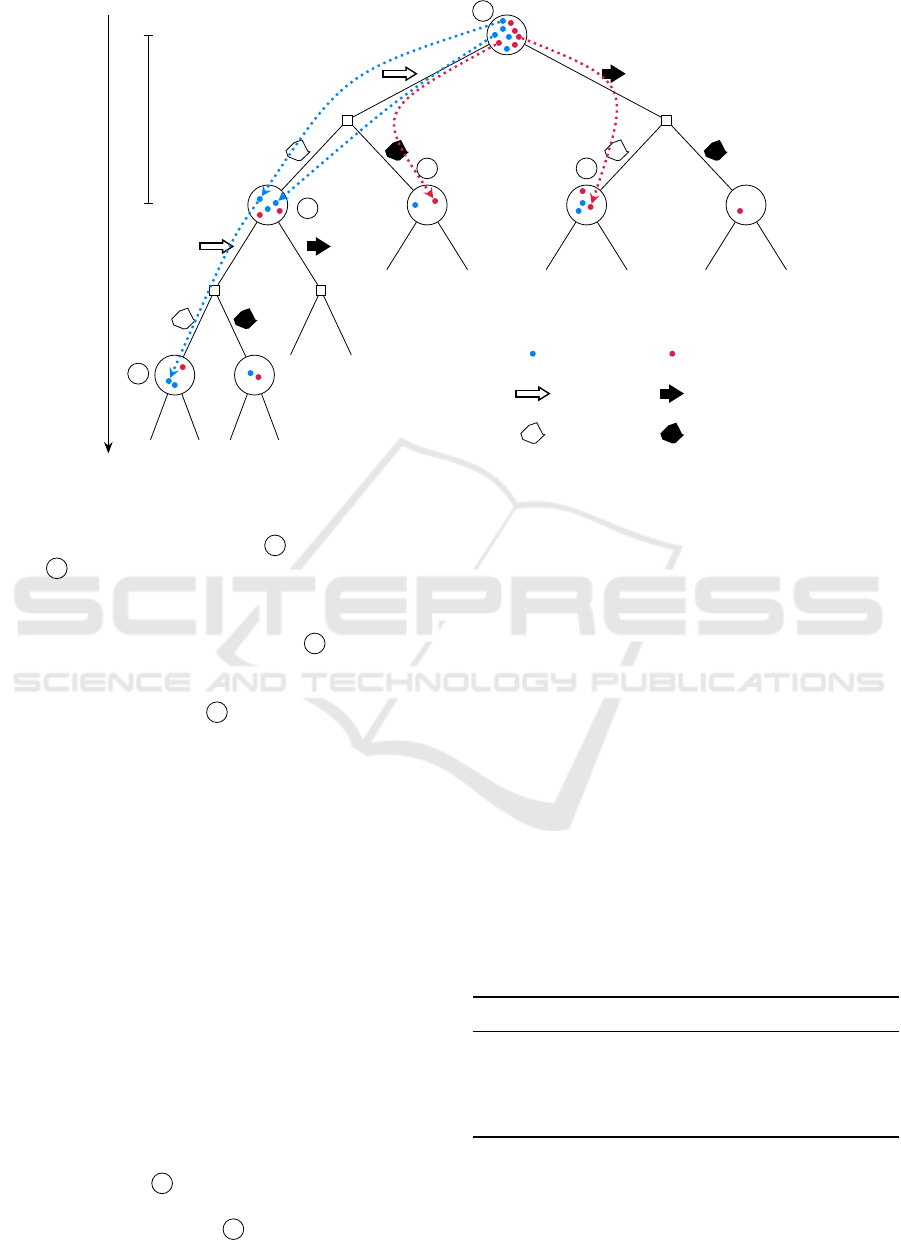
Belief b
0
planning horizon
∆t
state with no
obstacle
state with
obstacle
action
acceleration
action
deceleration
observed
no obstacle
observed
obstacle
1
2
3
4
5
Figure 3: Simplified belief tree with several sampled episodes.
as observations cannot be controlled, the particle might
receive another observation as in
2
and land in belief
node
4
which terminates this episode.
5.
Assuming a low
c
UCT
, the algorithm might
choose to accelerate again for the fourth particle. Do-
ing so, the particle might reach belief
2
which is not
new this time. Thus, the episode is extended and a
second action is selected and a new observation made,
to end up for example at
4
. After each episode, the
values of the belief nodes are updated according to
(11)
. By this, the new information is passed up the
tree.
6.
The procedure is repeated for a predefined num-
ber of episodes
n
epis
(here: 5000) or until a given time
limit is reached. Running down deeper into the tree,
eventually particles with a different obstacle state will
be separated by observations and land in different be-
lief nodes: A particle containing an obstacle is more
likely to cause a positive observation and vice versa.
This way, the POMDP factors in future information
gain.
7.
Now the agent has to decide for the real action.
Instead of deciding after the UCT in
(9)
which rewards
exploration, it chooses the action that maximizes the
(approximated) Q-function
ˆ
Q(b,a)
in
(11)
, thus, ex-
ploiting the information in the tree. Afterwards, it
receives an actual observation. In our case, it might
decide to accelerate and see no obstacle. The corre-
sponding belief at
2
is picked as the new root of the
tree. All other branches of the former root can be
pruned. The subtree under
2
is kept. Keeping parts
of the tree between time steps is one of the key features
of ABT, rendering it more efficient, as it does not have
to start from scratch in each step. Ideally, the parti-
cles in the new root belief form a better representation
of the actual state and the agent incrementally gets
“smarter”.
8.
Like all particle filters, also ABT suffers from
particle depletion. Particles explored with a different
action at the first step or having received wrong obser-
vations are lost. Eventually, after several time steps no
particle is left that fits the actual observation. To over-
come this problem, ABT offers a default implementa-
tion to replenish particles. It tries to “force” particles
from the previous belief into the new one by always
choosing the action actually performed and “hoping”
to receive the correct observation, until a minimum
number of particles
n
min,part
= 1000
is reached at the
new root. More efficient ways can be implemented by
the user.
Table 2: Parameters ABT.
Name Symbol Value Unit
UCT factor c
UCT
1000 -
Episodes per step n
epis
5000 -
Minimal particle count n
min,part
1000 -
Maximum depth - 20 -
VEHITS 2020 - 6th International Conference on Vehicle Technology and Intelligent Transport Systems
316
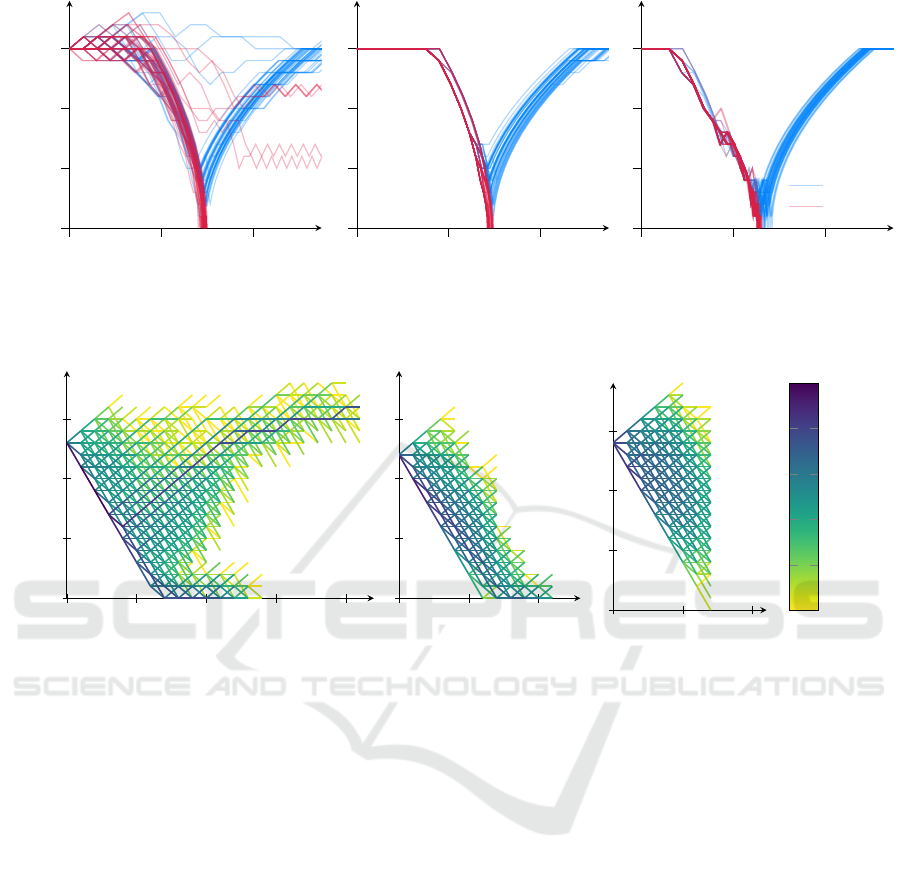
0 200 400
0
10
20
30
position [m]
velocity [m/s]
(a) c
UCT
= 1,
ˆ
Q
max
0 200 400
position [m]
(b) c
UCT
= 10
3
,
ˆ
Q
max
0 200 400
position [m]
no obstacle
obstacle
(c) c
UCT
= 10
3
,
ˆ
Q
default
Figure 4: 50 simulated trajectories for each ABT configuration with and without obstacle.
0
5
10
15
20
0
10
20
30
prediction time [s]
velocity [m/s]
(a) c
UCT
= 1
0
5
10
prediction time [s]
(b) c
UCT
= 10
3
0
5
10
prediction time [s]
10
0
10
0.2
10
0.4
10
0.6
10
0.8
10
1
number of episodes
(c) c
UCT
= 10
7
Figure 5: Explored actions of 5000 episodes with no obstacle and different UCT-factors, sampled at
t = 7 s
(simulation time).
The color shows the number of episodes passing along the edge on a logarithmic scale. On the negative part of the prediction
time, the trajectory taken so far is shown.
3.3 Analysis
The algorithm is analyzed in a small simulation envi-
ronment of the above example. It uses the same models
for state transition and observations as the POMDP
model in Sec. 3.1. For real-life applications, this is
a strong assumption and it would be safer to add ar-
tificial noise to both parts of the POMDP model to
make ABT more robust. For our simulation, this is not
needed.
Due to the probabilistic part of the observation
function, both the “real” observations and the con-
struction of the tree are non-deterministic. To enable a
reliable evaluation, each parameter set was simulated
50 times. The resulting trajectories of three configura-
tions are shown in Figure 4. The first, in Figure 4a, is
an example for choosing
c
UCT
too low. The algorithm
does not explore enough, subsequently in some cases
it does not see the possibility of a crash and does not
sufficiently reduce the velocity. In case of an obstacle
(red) it then fails to stop in front of the obstacle at
300 m. After the crash, the reward function is domi-
nated by the crash penalty so that the agent behaves
irrationally.
Choosing an appropriate
c
UCT
results in a much
more consistent behavior, as in Figure 4b. The agent
shows the expected behavior, it slows down in front of
the potential obstacle and once it is certain that there
is no threat, it accelerates again. The point of acceler-
ating again depends on the sequence of observations
made. In Figure 4c the default Q-function from
(10)
with equal
c
UCT
is shown. Notice the more conserva-
tive behavior causing it to brake much earlier.
The effect of the UCT-factor can also be seen when
looking at the belief tree; compare Figure 5a and Fig-
ure 5b. Both show the velocity curves of the sampled
episodes in one planning step in one of the simulations.
The exact tree highly depends on the observations
made, therefore they are not directly comparable. Yet,
it is obvious that a lower
c
UCT
leads to more selective
Tutorial on Sampling-based POMDP-planning for Automated Driving
317
10
0
10
1
10
2
10
3
10
4
10
5
10
6
10
7
0
500
1000
1500
6×crash 4×crash 43×crash
UCT factor
total cost (negative reward)
no obstacle
obstacle
mean & std.dev.
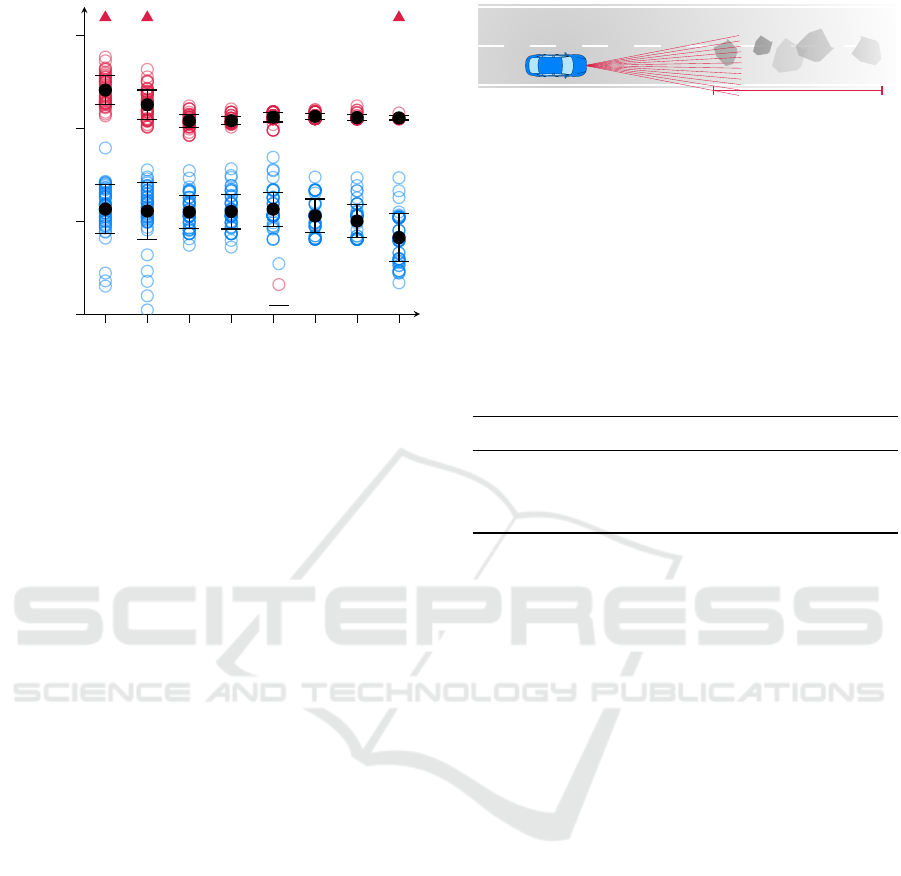
Figure 6: Total negative rewards of the simulations with
mean and standard deviation. Crashes are excluded but
shown at the top and lie in the range of 10
6
.
exploration. The plan of slowing down for another 4 s
and then speeding up again is clearly visible. On the
plus side, the algorithm may focus on more promis-
ing regions of the tree. On the downside, it samples
the edges less often and therefore might not encounter
unlikely but disastrous observations.
This leads to another effect: A higher
c
UCT
leads
to a shorter planning horizon. The reason being that,
as all branches of the tree are explored more evenly,
less episodes reach to a deeper level in the tree, as
can be seen in Figure 5c. If the planning horizon falls
below the time needed to make a stop, crashes cannot
be prevented. Notice the higher velocity at the root
node, indicating a more aggressive driving.
The final evaluation of the reached rewards with
different UCT factors is shown in Figure 6. Due to the
stochastic character of the observations both in build-
ing the tree and in the actual observations received, the
results vary. Therefore, 50 Simulations were carried
out with each configuration. The results confirm the
deductions: A too low UCT-factor leads to too op-
timistic behavior, approaching the potential obstacle
too fast and not being able to prevent crashes in all
cases. Setting
c
UCT
too high, in turn, leads to a too
short horizon and many crashes.
4 SCENARIO: CONTINUOUS
CASE
The scenario from above is now extended in that the
position of the potential obstacle is no longer known.
The new scenario is depicted in Figure 7. The agent
Figure 7: The position of the obstacle is no longer fixed but
the agent expects it to lie in the marked area.
expects the obstacle to lie within a 2 km stretch starting
at
x
p,start
. The obstacle is not guaranteed to exist. As
in the Binary Case, there may be no obstacle at all. All
other aspects of the scenario are left untouched: Except
for the obstacle position, all parameters from Table 1
are still valid. Within the simulation, the obstacle is
always placed at the same position (if existing) without
loss of generality. The new parameters are listed in
Table 3.
Table 3: Parameters for the Continuous Case.
Name Symbol Value Unit
Obstacle zone start x
p,start
300 m
Obstacle zone end x
p,end
2300 m
Actual position x
p
500 or
/
0 m
4.1 Model Changes
The new scenario has to be represented by changes in
the model. In the following, the affected components
of the POMDP as in (1) are mentioned.
States S:
In addition to the vehicle states and the
obstacle existence, the new state also encompasses
the obstacle position
x
p
as a hidden variable:
s =
x
v
,v
v
,e
p
,x
p
|
. While the vehicle states have been
continuous already, the new state variable also renders
the unobservable part continuous, adding complexity
to the problem.
Possible Observations O:
When close enough, the
agent may perceive the distance
d
meas
to the obstacle
and can deduce its position. Therefore, observations
now consist of two components:
o
0
= (o, d
meas
)
|
with
the observed existence o ∈ {0,1} already introduced.
Observation Function Z:
The probability functions
for observing the obstacle existence
P(o|e
p
)
remain
unchanged as in
(3)
and
(4)
. Note that this still allows
for false positives. Additionally, the distance measure-
ments have to be included. For sake of simplicity, we
assume that the distance is correctly measured if a pos-
itive existence measurement is received. Otherwise,
the laser hits nothing and
d
meas
is simply set to the
range of vision d
view
.
d
meas
=
(
x
p
− x
v
for o = 1,
d
view
else .
(12)
VEHITS 2020 - 6th International Conference on Vehicle Technology and Intelligent Transport Systems
318
Initial Belief b
0
:
As in the previous case, the agent
has to make assumptions about the hidden states before
the start. We stick to the 50 % chance that there is an
obstacle at all. For the obstacle position, it is assumed
to lie within the interval from
x
p,start
to
x
p,end
. That
means that the obstacle positions for the particles in
b
0
are drawn from an uniform distribution. By default,
particles are drawn using a random generator. Here,
we enforced an actually uniform distribution by evenly
placing the obstacles over the interval, which slightly
increases the reproducibility. The initial distribution
can also be seen in Figure 8.
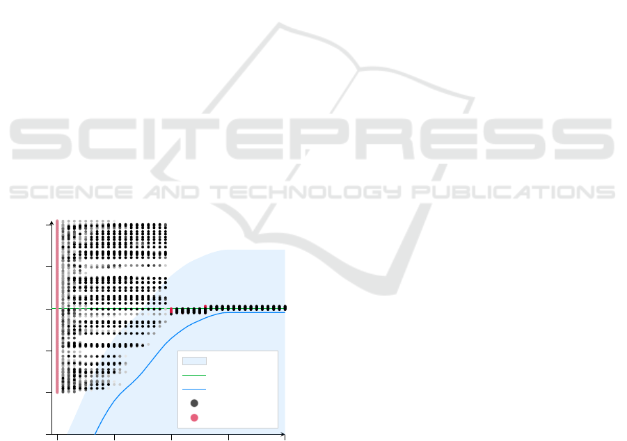
4.2 Complications in Solving
The continuous observations and continuous hidden
states pose problems for the ABT algorithm. We will
analyze those problems looking at Figure 8. On the
left at 0 s the uniform distribution of the particles can
be seen. Note that only those particles are shown that
contain an obstacle (
e
p
= 1
). As all particles are freshly
sampled, they are highlighted in red. At this point the
agent (blue) is still far away, its field of vision does not
reach the potential obstacle positions, yet. Therefore,
the agent gained no information.
4.2.1 Particle Depletion
Still, because ABT only keeps those particles that took
the same action and received the same observation,
inherently, particles get lost, because they were not
0 10 20 30 40
200
300
400
500
600
700
time [s]
position [m]
field of vision
actual obstacle
agent
old particles
new particles
Figure 8: The potential obstacle positions in the particle filter
are shown over the course of a simulation. For reference, also
the agent, its field of view and the actual obstacle position are
shown. When the agent gets closer to the particle positions,
negative observations make their existence less likely. When
the agent receives the first positive measurement at 20 s, it is
able to brake in time. c
UCT
= 10
3
.
‘lucky’ enough to land in the right belief. This equals
a loss of information. The so-called particle deple-
tion is a common problem for particle filters but es-
pecially severe with the ABT and continuous states.
The reason being, that the ABT does not perform reg-
ular resampling as it tries to keep the subtree, while
moving or generating new particles would mean to
loose their episodes. This behavior is opposed to the
DESPOT solver which uses an independent conven-
tional particle filtering algorithm including importance
resampling (Thrun et al., 2005).
This problem aggravates with increasing domain
size. The larger the state space, the more particles are
required for an adequate representation. Especially
further dimensions (e.g., a moving obstacle) or infinite
domains (obstacle position not restricted) will lead to
failure without special consideration.
The effect of particle depletion can be seen at 20 s
in Figure 8 when the agent receives its first positive
measurement. At this point hardly any particles are
close to the observed position. Therefore, emergency
resampling is started, which creates particles close to
the observed location. Obviously that is very ineffi-
cient as the tree has to be re-calculated almost from
scratch.
4.2.2 Infinite Branching Factor
Another problem arises from the continuous obser-
vations. All three algorithms, ABT, POMCP and
DESPOT, were designed for discrete observations (and
actions). Whenever a new observation is made, a new
observation branch and subsequent belief are opened
up. In case of continuous observation this would mean
that each particle lands in its own belief, degenerat-
ing the tree just after one step. There are methods to
counteract this issue, one of them being progressive
widening (Cou
¨
etoux et al., 2011) which artificially
limits the number of available observations at each ac-
tion node, forcing episodes to run deeper into the tree.
Progressive widening and its drawbacks are analyzed
in (Sunberg and Kochenderfer, 2018).
Another option, that may also be activated in ABT,
is to use discretization. Here, two observations are con-
sidered equal if a certain distance function falls below
a preset threshold. In that case, the episode is routed
into the same belief. If the considered particle may not
be assigned to any existing belief, a new belief node is
set up. If several beliefs are possible, the episodes pick
the closest belief according to the distance function.
One possible distance function uses the observed
existence and distance:
Tutorial on Sampling-based POMDP-planning for Automated Driving
319
∆(o
i
,o
j
) =
0 if o
i
= 0 ∧ o
j
= 0,
d
meas,i
− d
meas, j
if o
i
= 1 ∧ o
j
= 1,
∞ else
(13)
When both observations are negative, they are consid-
ered equal. If both are positive, the observations are as
far apart as the observed distances. If the existence ob-
servations differ, they must not be equal. The equality
is determined by
∆(o
i
,o
j
) ≤ ∆
max
. (14)
Now, the threshold
∆
max
plays an important role, in
addition to the UCT-factor in the Binary Case. The
results of different parameter choices are shown in Fig-
ure 9. Two effects can be seen: When the maximum
distance is chosen small, the algorithm can precisely
react to the observation, resulting in general in lower
costs. On the other hand, a low maximum distance
leads to narrow and therefore many belief nodes, corre-
sponding with a fine-grained but not deep search tree.
In the extreme case at
∆
max
= 1m
, the horizon is too
short, such that braking in time is not always possible.
On the other end, greater distances allow for less
observation branches and deeper trees, but they face
another problem: If a belief stretches over a large
section, there may be trajectories passing through that
belief and not crashing, even though the obstacle lies
within that section. The reason being, that the obstacle
is simply ‘further behind’ within the section spanned
by the belief. In such a case, the belief may receive a
good value estimate, making it attractive, even though
it is dangerous. The resolution is simply too coarse.
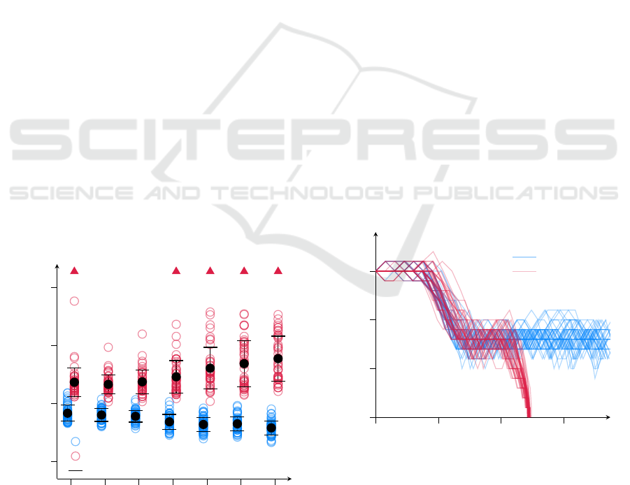
1 5 10 20 30 40 50
500
1000
1500
2000
2×crash 5×crash 7×crash 5×crash 6×crash
max. observation distance [m]
total cost (negative reward)
no obstacle
obstacle
mean & std.dev.
Figure 9: Total negative rewards of the simulations with
different maximum observation distances. Crashes are again
shown at the top. Each configuration was simulated 50 times.
c
UCT
= 10
3
.
4.2.3 Short Horizon
Hand in hand with the above issue goes the problem of
a too short horizon. As there are more possible obser-
vations, the branching factor is increased, the tree gets
wider and shallower. With
n
epis
= 5000
episodes, the
algorithm only reaches a planning horizon of 6-7 steps.
As already shown in Figure 5c and Figure 6, that is not
enough to prevent crashes. And indeed, the algorithm
crashes often when used in this configuration. For that
reason we make use of the heuristic already mentioned
in Step 2 in Section 3.2. The heuristic is called when
an episode hits a new belief node. It returns a first
estimate for the value of the belief. As a heuristic
we use the Intelligent Driver Model (IDM) (Treiber
and Kesting, 2013) in a discretized version (acceler-
ations are rounded to the available actions in
A
, see
Section 3.1). The situation in the particle (including
hidden states) is simulated forward until the planning
horizon (20 steps) using the accelerations of the IDM
as actions for the agent. This helps to detect beliefs
that inevitably crash into the obstacle and should be
avoided; the horizon is artificially prolonged.
Using the heuristic and choosing UCT-factor and
maximum observation distance wisely leads to a rea-
sonable behavior as in Figure 10. Before the agent
enters the potential obstacle zone starting at 300 m, it
has already reduced its velocity. When the obstacle
appears at
x
p
= 500 m
, the agent is slow enough to pre-
vent a crash in all cases. When there is no obstacle, the
agent continues with lowered speed until the danger
zone is left.
0 200 400
600
0
10
20
30
position [m]
velocity [m/s]
no obstacle
obstacle
Figure 10: Simulated trajectories with the obstacle position
unknown to the agent. 50 runs each for no obstacle and
obstacle at
x
p
= 500m
. The potential obstacle zone starts at
x
p,start
= 300 m
. As the agent reduces its velocity sufficiently
in advance, it never crashes. The fluctuation in velocity is
due to under-sampling. There are not enough episodes to
reproduce the fine difference in the cost function.
VEHITS 2020 - 6th International Conference on Vehicle Technology and Intelligent Transport Systems
320

5 CONCLUSION & OUTLOOK
In this work we presented the scenario of an uncer-
tain obstacle in automated driving. The example was
used to motivate and explain the use of POMDPs. We
derived its components and explained the functional-
ity of the ABT solver. Even though the chosen sce-
nario was kept simple, it is complex enough to point
out five different difficulties that have to be overcome
when trying to solve a real world problem. At the
simpler scenario with a fixed obstacle position, we
demonstrated the impact of the UCT-factor, balancing
exploration versus exploitation, and suggested using a
suitable estimate for the Q-value-function. Extending
the scenario to include continuous hidden states and
observations brought further problems. Namely, we
could show the need for discretizing observations in
order to prevent a degenerated tree, and pointed at the
influence of the particle filter. Lastly, the advantage of
using a heuristic function as a first estimate for a belief
value was explained.
Even though we did not solve a burning problem
in this work, we hope to pave the way for others into
POMDP-based behavior planning by bringing insights
into the mechanisms. Especially at the advent of paral-
lelizing solver algorithms (Cai et al., 2018), promising
to alleviate the massive drawback of the computational
burden, we expect to find POMDPs in more and more
applications. Apart from speeding up the algorithms,
we see need for further research in handling continuous
observations. Perhaps, smart discretization combined
with progressive widening may help in that regard.
ACKNOWLEDGMENT
This research was supported by AUDI AG.
REFERENCES
Cai, P., Luo, Y., Hsu, D., and Lee, W. S. (2018). Hyp-despot:
A hybrid parallel algorithm for online planning under
uncertainty.
Cou
¨
etoux, A., Hoock, J.-B., Sokolovska, N., Teytaud, O.,
and Bonnard, N. (2011). Continuous upper confidence
trees. In International Conference on Learning and
Intelligent Optimization, pages 433–445. Springer.
Gonz
´
alez, D. S., Garz
´
on, M., Dibangoye, J., and Laugier,
C. (2019). Human-like decision-making for automated
driving in highways. In 2019 IEEE 22nd Interna-
tional Conference on Intelligent Transportation Sys-
tems (ITSC).
Hubmann, C., Quetschlich, N., Schulz, J., Bernhard, J., Al-
thoff, D., and Stiller, C. (2019). A pomdp maneuver
planner for occlusions in urban scenarios. In 2019
IEEE Intelligent Vehicles Symposium (IV), pages 2172–
2179.
Hubmann, C., Schulz, J., Becker, M., Althoff, D., and Stiller,
C. (2018a). Automated driving in uncertain environ-
ments: Planning with interaction and uncertain ma-
neuver prediction. IEEE Transactions on Intelligent
Vehicles, 3(1):5–17.
Hubmann, C., Schulz, J., Xu, G., Althoff, D., and Stiller, C.
(2018b). A belief state planner for interactive merge
maneuvers in congested traffic. In 2018 IEEE 21st
International Conference on Intelligent Transportation
Systems (ITSC), pages 1617–1624.
Klimenko, D., Song, J., and Kurniawati, H. (2014). Tapir: A
software toolkit for approximating and adapting pomdp
solutions online. In Proceedings of the Australasian
Conference on Robotics and Automation, Melbourne,
Australia, volume 24.
Kocsis, L. and Szepesv
´
ari, C. (2006). Bandit based monte-
carlo planning. In European conference on machine
learning, pages 282–293.
Kurniawati, H. and Yadav, V. (2016). An online pomdp
solver for uncertainty planning in dynamic environ-
ment. In Robotics Research, pages 611–629. Springer.
Papadimitriou, C. H. and Tsitsiklis, J. N. (1987). The com-
plexity of markov decision processes. Mathematics of
operations research, 12(3):441–450.
Russell, S. J. (1998). Learning agents for uncertain environ-
ments. In COLT, volume 98, pages 101–103.
Sch
¨
orner, P., T
¨
ottel, L., Doll, J., and Z
¨
ollner, J. M. (2019).
Predictive trajectory planning in situations with hidden
road users using partially observable markov decision
processes. In 2019 IEEE Intelligent Vehicles Sympo-
sium (IV), pages 2299–2306.
Silver, D. and Veness, J. (2010). Monte-carlo planning
in large pomdps. In Advances in neural information
processing systems (NIPS), pages 2164–2172.
Somani, A., Ye, N., Hsu, D., and Lee, W. S. (2013).
Despot: Online pomdp planning with regularization.
In Advances in neural information processing systems
(NIPS), pages 1772–1780.
Sunberg, Z. N. and Kochenderfer, M. J. (2018). Online
algorithms for pomdps with continuous state, action,
and observation spaces. In Twenty-Eighth International
Conference on Automated Planning and Scheduling.
Thrun, S., Burgard, W., and Fox, D. (2005). Probabilistic
robotics. MIT press.
Treiber, M. and Kesting, A. (2013). Traffic Flow Dynamics:
Data, Models and Simulation. Springer.
Ye, N., Somani, A., Hsu, D., and Lee, W. S. (2017). Despot:
Online pomdp planning with regularization. Journal
of Artificial Intelligence Research, 58:231–266.
Tutorial on Sampling-based POMDP-planning for Automated Driving
321
