Polygonal Meshes of Highly Noisy Images based on a New Symmetric
Thinning Algorithm with Theoretical Guarantees
Mohammed Arshad Siddiqui
1 a
and Vitaliy Kurlin
2 b
1
PDPM Indian Institute of Information Technology Design and Manufacturing, Jabalpur, India
2
University of Liverpool, U.K.
Keywords:
Edge Detection, Thinning, Skeletonization, Polygonal Mesh.
Abstract:
Microscopic images of vortex fields are important for understanding phase transitions in superconductors.
These optical images include noise with high and variable intensity, hence are manually processed to extract
numerical data from underlying meshes. The current thinning and skeletonization algorithms struggle to find
connected meshes in these noisy images and often output edge pixels with numerous gaps and superfluous
branching point. We have developed a new symmetric thinning algorithms to extract from such highly noisy
images 1-pixel wide skeletons with theoretical guarantees. The resulting skeleton is converted into a polygonal
mesh that has only polygonal edges at sub-pixel resolution. The experiments on over 100 real and 6250
synthetic images establish the state-of-the-art in extracting optimal meshes from highly noisy images.
1 INTRODUCTION
Microscopic image analysis of topological defects
(called quantum vortices) in symmetry-breaking
phase transitions is now a hot topic in cosmology
and high-temperature superfluids and superconduc-
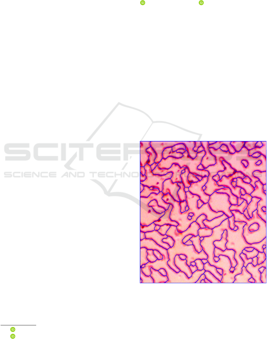
tors (Lin et al., 2014). Figure 1 shows a piezo-
response force microscopic image of a vortex field.
The underlying vortex field is a complicated mesh of
non-convex polygons that is hard to recognize even by
human experts because of the highly variable noise.
To understand phase transitions, physicists ur-
gently need to count various statistics of vortex fields
such as the number and positions of vertices, the num-
ber and sizes of polygonal domains. Since past algo-
rithms produced incomplete meshes with discontinu-
ities or hanging endpoints, see section 6, human ex-
perts had to manually count features of vortex images.
This paper automates the collection of statistical data
that will enable a discovery of high-temperature su-
perconductors as motivated in (Lin et al., 2014).
Definition 1. A vortex mesh on an image Ω is a skele-
ton or an embedded graph splitting Ω into domains
with polygonal edges that consist of straight line seg-
ments and meet at vertices of degree at least 3.
a
https://orcid.org/0000-0002-9747-3132
b
https://orcid.org/0000-0001-5328-5351
Figure 1: Our new mesh on top of a typical microscopic im-
age, see high resolution images in supplementary materials.
Optimal Mesh Problem. For any highly noisy vor-
tex image as in Figure 1, find a connected polygonal
mesh that minimizes the average intensity (to get a
darkest skeleton) and has a minimum number of ver-
tices.
Siddiqui, M. and Kurlin, V.
Polygonal Meshes of Highly Noisy Images based on a New Symmetric Thinning Algorithm with Theoretical Guarantees.
DOI: 10.5220/0009340301370146
In Proceedings of the 15th International Joint Conference on Computer Vision, Imaging and Computer Graphics Theory and Applications (VISIGRAPP 2020) - Volume 4: VISAPP, pages
137-146
ISBN: 978-989-758-402-2; ISSN: 2184-4321
Copyright
c
2022 by SCITEPRESS – Science and Technology Publications, Lda. All rights reserved
137
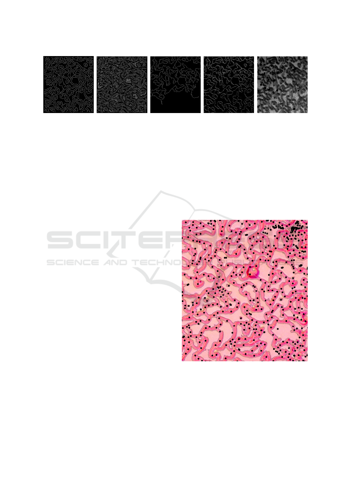
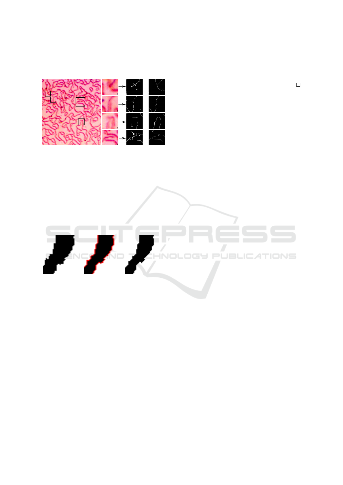
Figure 2: Past edge detection on the input in Figure 1. 1st: many disjoint components based on a small number of Canny
edge pixels (Canny, 1986). 2nd: many superfluous components based on a large number of Canny edge pixels. 3rd: fuzzy
logic skeletonization (Kamani et al., 2018). 4th: (Asghari and Jalali, 2015). 5th: watershed by (Soille and Vincent, 1990).
The primary minimization is for the average in-
tensity, because the underlying vortex mesh is rep-
resented by darker pixels. The secondary minimiza-
tion is for the number of degree 2 vertices to simplify
polygonal lines between higher degree vertices.
Here are the challenges in solving the above problem
for the highly noisy microscopic images in practice.
• Polygonal lines have a large and variable thickness
and can meet at higher degree vertices at any angle.
• The intensity largely varies and leads to many noisy
edges, compare with a ground truth in Figure 18.
• Microscopic images often contain isolated noisy
blobs that should be ignored and also larger blobs that
should be treated as vertices or parts of lines.
Here are the novelty and contributions of the paper. to
the state-of-the-art skeletonization of noisy images.
• New Definition 5 formalizes a 1-pixel wide skeleton
guaranteed in the output by Theorem 6.
• The new erosion algorithm in section 4 preserves the
homotopy type (stronger than a graph connectivity)
for any binary image, see Definition 3, Theorem 8.
• Table 1 in section 6 shows that our thinning out-
performs all past algorithms on the minimum average
intensity on over 100 real images and also produces
simpler meshes without erroneous degree 1 vertices.
• Table 2 has standard accuracy measures averaged
over 6250 ground truths and shows that the new sym-
metric thinning in section 5 is robust under noise.
Here is the pipeline for the optimal mesh extraction.
Stage 1: the Otsu thresholding (Otsu, 1979) is
adapted for microscopic images with variable noise
in section 3 to get a connected binary image.
Stage 2: any binary image is symmetrically thinned
to a 1-pixel wide skeleton without degree 1 vertices,
see proofs of Theorems 6 and 8 in section 4.
Stage 3: a 1-pixel wide skeleton from Stage 2 is con-
verted to a mesh whose polygonal lines are further
straightened for a statistics analysis in section 6.
2 A REVIEW OF PAST WORK
Edge Detection Algorithms. The Canny edge de-
tector (Canny, 1986) depends on 3 thresholds and can
output many disjoint components, see Figure 2.
Morse-Smale skeleton (Delgado-Friedrichs et al.,
2014) consists of gradient flow curves joining local
extrema and saddle points of the grayscale intensity.
Figure 3 shows a Morse-Smale skeleton with many
superfluous black vertices joined by white curves.
Figure 3: The Morse-Smale skeleton (Delgado-Friedrichs
et al., 2014) with black dots for local minima and saddles.
The recent survey on skeletonization (Saha et al.,
2016) is a comprehensive review of past approaches
and current challenges. Typical requirements for a
skeleton representing a binary (black-and-white) im-
age is (1) centrality, (2) invariance under rotations and
other deformations, (3) connectedness or preservation
of a topological type (Kurlin, 2015a), (Kurlin, 2015b),
VISAPP 2020 - 15th International Conference on Computer Vision Theory and Applications
138
(Kalisnik et al., 2019), (Smith and Kurlin, 2019).
Another aim from Bernard in (Bernard and Man-
zanera, 1999) is to guarantee that a skeleton is 1-pixel
wide, because a big block of black pixels such as
(Saha et al., 2016, Figure 1) or Figure 11 is an obsta-
cle for many thinning algorithms. The new thinning
algorithm in sections 4-5 solves problem by introduc-
ing a 1-pixel wide skeleton in Definition 5.
OpenCV offers the thinning by (Zhang and Suen,
1984) and (Guo and Hall, 1989). Both methods use
a 3 × 3 neighborhood to decide which pixels to re-
move. The first method (Zhang and Suen, 1984) con-
sists of two sub-iterations where the pixels are re-
moved from north-east and south-west corners, then
from the south-east and north-west corners. The sim-
ilar second method guarantees (Guo and Hall, 1989,
Proposition A.3) the global connectivity of clusters,
not the homotopy type in Definition 3, so a circular
cluster can become a non-closed polygonal line.
Fuzzy Logic: Kamani (Kamani et al., 2018) proposed
a skeletonization method based on fuzzy logic, which
can take any grayscale image, see Figure 2(3).
CNNs: convolutional neural networks (Wang et al.,
2018), (Shen et al., 2017), (Panichev and Voloshyna,
2019) were particularly successful in cases when a lot
of ground truth data is available, see Fig. 4.
Figure 4: The output by (Asghari and Jalali, 2015) on the
image from Figure 1. One could zoom in and find many
disjoint components instead of one big connected skeleton.
3 THE NEW ADAPTIVE
THRESHOLDING
This section discusses Stage 1 of the proposed solu-
tion to the Optimal Mesh Extraction Problem from
section 1. Since a mesh is still detectable by hu-
man eye in grayscale, the mesh problem was stated in
terms of minimizing the average grayscale intensity.
Stage 1 will build a connected binary image.
Definition 2. For a given width w and height h, a
binary image on the continuous domain Ω = [0,w] ×
[0,h] ⊂ R
2
is a set of black unit square pixels whose
complement in Ω consists of the white unit square pix-
els in the background. An image I is connected if the
union of its black pixels forms a connected sub-graph
in the 8-connected grid of Ω.
We have tried many thresholdings to get a con-
nected image that can be further thinned. Our micro-
scopic images have uneven illumination with darker
regions towards the image boundary. This gradual
change in intensity was not uniform in given images.
The global and local thresholding methods (Bernsen,
1986), (Niblack, 1985), (Phansalkar et al., 2011),
(Sauvola and Pietik
¨
ainen, 2000), (Soille, 2013) often
fail to preserve continuity of edges in the noisy im-
age from Figure 1, see outputs of above binarizations
in Figure 6. The clustering-based thresholding (Otsu,
1979) couldn’t find an optimal threshold. Figure 5
shows the Otsu thresholding with many components.
To resolve uneven illumination, we find optimal
parameters for Otsu binarization in sub-images of size
M × M within 2584× 1936 images. Otsu binarization
chooses an optimal threshold using the histogram of
all intensities. Since some sub-images are dark, we
shift any intensity i lower than a certain bound b for
all sub-images by i 7→ (i + b)/2.
The parameters M and b are dynamically selected
for each image as follows. The original image is di-
vided into M × M sub-images whose average inten-
sities are calculated. The value of M increases from
50 to 400 in increments of 25. We choose M so that
the standard deviation of the average intensity in sub-
images is minimal. Then b is set as the average in-
tensity of the optimal sub-image. This shift implicitly
increases the optimal Otsu threshold and yields a con-
nected binary image in Figure 5 (middle).
A resulting image can have small holes as in the
middle of Figure 5, green box. Physicists advised us
that expected domains have at least 50 pixels, so we
have filled all small holes as in the right picture of
Figure 5, instead of the persistence-based hole detec-
tion (Kurlin, 2014b), (Kurlin, 2014a), (Kurlin, 2016).
The output of Stage 1 in Figure 5 (right) has few small
black components, which are removed in sections 4-5.
Polygonal Meshes of Highly Noisy Images based on a New Symmetric Thinning Algorithm with Theoretical Guarantees
139
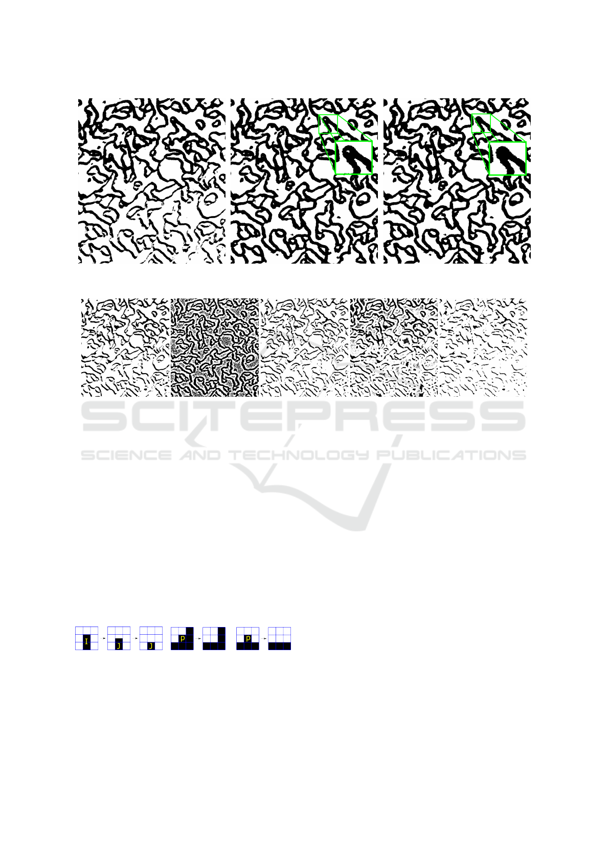
Figure 5: Left: original Otsu thresholding (Otsu, 1979) breaks connectivity in Figure 1. Middle: the new adaptive threshold-
ing outputs a better connected image, compare the bottom parts. Right: output of Stage 1 after filling small holes.
Figure 6: Outputs of several local thresholding methods on the input image in Figure 1. 1st: (Bernsen, 1986), 2nd: (Niblack,
1985), 3rd: (Phansalkar et al., 2011), 4th: (Soille, 2013) and 5th: (Sauvola and Pietik
¨
ainen, 2000).
4 THE NEW EROSION WITH
GUARANTEES
The output of Stage 1 is a binary image that covers
polygonal lines of a required vortex mesh. The next
stage is to thin (or erode) the binary image to preserve
its homotopy type without making any holes.
Definition 3. A subimage of a binary image I con-
sisting of black pixels on a continuous domain Ω is a
subset J ⊂ I of black pixels considered on the same
domain Ω of I. A homotopy (or a deformation re-
traction) f : I → J is a continuous family of functions
f
t
: Ω → Ω, t ∈ [0,1], such that f
0
= id
Ω
, f
1
= f and
all f
t
keep the points of J fixed.
Figure 7: A homotopy
of an image I to its
subimage J is a contin-
uous deformation.
Figure 8: Examples of Erosion 2
when we remove a pixel p with
two changes of colors in neigh-
bors from Definition 4.
A homotopy can be visualized as a sequence of
pixel removals that preserve the topological shape
of a binary image. A removal of a pixel with only
one neighbor (in the 3 × 3 neighborhood) is a homo-
topy by Definition 3. A removal of a pixel whose
two neighbors become disconnected (as formalized in
Definition 4) cannot be realized by a continuous fam-
ily of deformations, so isn’t a homotopy.
Definition 4. (neighbors) Any non-boundary black
(foreground) pixel p has 8 neighbors in the 3 × 3-
neighborhood. Any white (background) pixel has only
4 neighbors. When we walk around the pixel p (say,
clockwisely starting from any neighbor), we count the
number of color changes in the 8 neighbors of p from
black to white and from white to black.
Section 5 describes the new algorithm that sym-
metrically removes pixels starting from an external
layer and outputs a better skeleton with a lower av-
erage intensity. We now discuss a simpler thinning
when pixels are removed one by one being processed
from top to bottom and from left to right.
Erosion 1. Remove a black pixel that has at most 1
neighbor, e.g. any isolated pixel is removed as an out-
lier. We remove pixels with 1 neighbor as in Figure 7
since a vortex mesh has no degree 1 vertices.
VISAPP 2020 - 15th International Conference on Computer Vision Theory and Applications
140
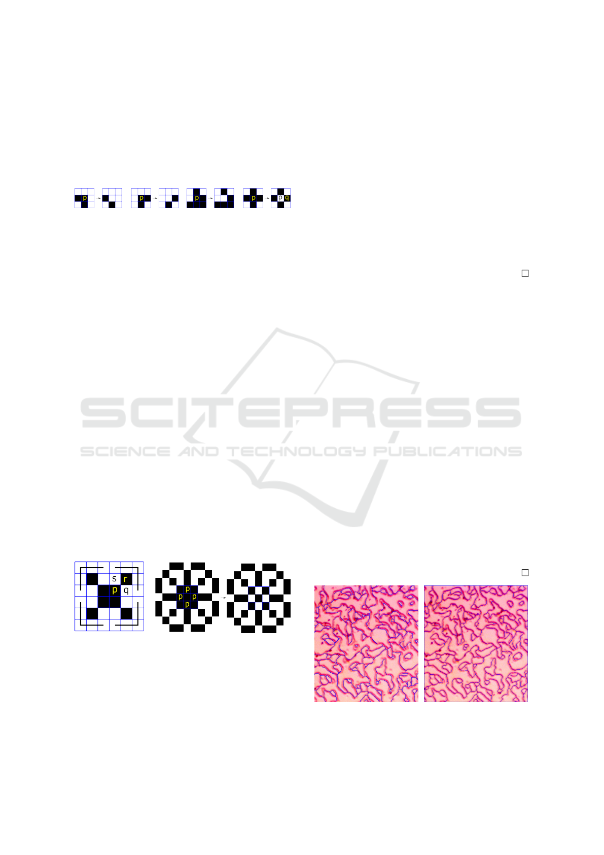
Erosion 2. Remove a black pixel p if colors change
twice around p, see Definition 4 and Figure 8.
Erosion 3. Remove a black pixel p if p has 4
changes of colors, but all its neighbors are pairwise
adjacent to each other in the 8-connected grid, see
Figure 9.
Figure 9: Erosion 3 removes
a pixel p with four changes
of colors. in neighbors.
Figure 10: Erosion 4 re-
moves a pixel p when all
black neighbors are con-
nected.
Erosion 4. We remove a black pixel p if p wasn’t
removed by any of Erosions 1-3, p has at least two
white neighbors and all its black neighbors form a
connected sub-graph (in the 8-connected grid), see
Figure 10. This erodes busy junctions as in Fig-
ure 11 (right), which were obstacles for homotopy-
preserving thinning (Saha et al., 2016). Erosion 3 was
separated from Erosion 4 to speed up the algorithm.
The erosion algorithm scans a binary image row by
row, processing black pixels in each row from left to
right. Black pixels are stored in a map-structure for
quick access by a pixel position. For any black pixel,
we try Erosions 1,2,3,4 in this order until all remain-
ing pixels cannot be removed by Erosions 1-4.
New Erosion 4 resolves busy junctions to get a 1-
pixel wide skeleton (see Theorem 6) and keeps the ho-
motopy type of a binary image (modulo 1-pixel holes)
due to Theorem 8. Theorems 6 and 8 are two ‘edges
of the thinning sword’ justifying wider applications of
the thinning based on Erosions 1-4.
Definition 5. A binary image I consisting of black
pixels is called a 1-pixel wide skeleton if any 2 × 2
block contains at most 3 black pixels of I except the
case in Figure 11 (left), where each of 4 black pixels
has a diagonal neighbor.
Figure 11: Left: the 2 × 2 block cannot be removed because
of 4 diagonal neighbors. Right: Erosion 4 removes 4 pixels
p in the previously unresolved junction (Saha et al., 2016).
The diagonal neighbors in Figure 11(left) might
be kept by Erosions 1-4 if each of 4 black corner lines
contains at least one black pixel. Figure 11(right)
shows the power of new Erosion 4, which can pen-
etrate big black blocks by creating only 1-pixel holes
that can be later filled if needed. Our microscopic im-
ages had no superfluous 1-pixel holes from Erosion 4.
Theorem 6. For any binary image I with fixed bound-
ary black (background) pixels, the algorithm based on
Erosions 1-4 outputs a 1-pixel wide skeleton.
Proof of Theorem 6. If I isn’t a 1-pixel wide skeleton,
we can find a 2 × 2 block B of black pixels adjacent
(by a side) to at least one white pixel q. The side
neighbor p ∈ B of q cannot be removed by Erosion 4
only if its side neighbor s is white and corner neighbor
r is black as in the left picture of Figure 11 so that r
becomes disconnected from other neighbors of p if
q is eroded. The other 3 pixels in B cannot be eroded
only if they have diagonal neighbors in Figure 11.
Definition 7. A 1-pixel hole in a binary image I of
black pixels is a white pixel sharing 4 sides with black
pixels, see the central white pixel in the last picture of
Figure 10. A connected component C of an image I is
trivial if C has no holes larger than 1-pixel holes.
Theorem 8. For any image I without trivial compo-
nents and 1-pixel holes, the erosion after filling 1-
pixel holes outputs a subimage homotopic to I.
Proof of Theorem 8. If a central black pixel p shares a
side with a white pixel, the removal of p is realized by
a homotopy in the sense of Definition 3, see Figure 7.
If p is eroded and the 4 neighbors sharing sides with
p are black, Erosion 4 was applied and p becomes a
1-pixel hole by Definition 7. Erosions 1-4 preserve
the local connectivity, i.e. the neighbors of p remain
connected in the 8-connected grid.
Each of the 4 side neighbors q of p in Figure 10
cannot be later eroded, otherwise the two corner black
pixels (sharing sides with p and corners with q) be-
come disconnected in the 3 × 3 neighborhood of q.
Hence p will keep all its 4 side neighbors and will re-
main a 1-pixel hole that will not affect the homotopy
type (after filling 1-pixel holes in J).
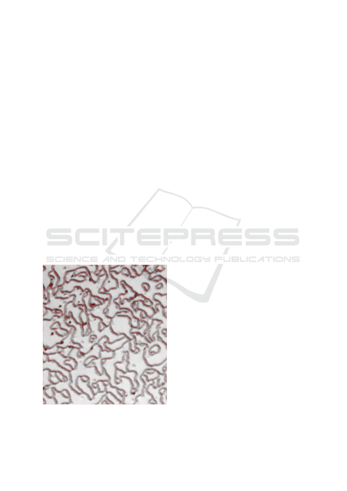
Figure 12: Ablation study: past thinning vs symmetrical.
Left: too straight lines after erosion in section 4. Right:
more accurate polygonal lines after symmetric thinning.
Polygonal Meshes of Highly Noisy Images based on a New Symmetric Thinning Algorithm with Theoretical Guarantees
141
5 SYMMETRIC THINNING AND
A MESH
Figure 13: Errors of past methods in subareas of Figure 1.
1st: extra edges (Zhang and Suen, 1984), 2nd: extra de-
gree 1 vertex (Guo and Hall, 1989), 3rd: lost connec-
tion (Arganda-Carreras et al., 2010), 4th: many superfluous
edges (Delgado-Friedrichs et al., 2014). Right: our mesh.
We improve the erosion algorithm from section 4 by
processing pixels not row by row, but in a data-driven
recursive way starting from the external layer.
Definition 9. For any binary image I ⊂ Ω consisting
of black pixels on a white background Ω − I, the ex-
ternal layer of I is the subset L ⊂ I of all black pixels
adjacent to a white pixel in the 4-connected grid.
Figure 14: The red external layer from Def. 9 is removed.
A continuous deformation of the image domain Ω
is any bijection Ω → Ω such that any adjacent pixels
(in the 8-connected grid of Ω) map to adjacent pixels.
Corollary 10. For any binary image I ⊂ Ω, the sym-
metric thinning algorithm outputs a skeleton S that is
invariant under any continuous deformation of Ω and
satisfies the conclusions of Theorems 6 and 8. Any
pixel of S has only 2 or 3 neighboring pixels in S.
The symmetric skeletons obtained from all our
microscopic images had no black 2× 2 blocks, which
were allowed in a 1-pixel wide skeleton from Defini-
tion 5. To guarantee that every skeleton has vertices
of only degrees 2 or 3, the final step of Stage 2 after
symmetric thinning is to resolve few cases of degree 4
vertices in Figure 15, which preserve connectivity in
5 × 5 or 6 × 6 neighborhood.
Proof of Corollary 10. The only difference between
the erosion algorithm in section 4 and the new sym-
metric thinning in Figure 14 is the order in which pix-
els are processed. Since Definition 9 uses adjacency
of pixels in the 4-connected grid, the output remains
the same under any continuous deformation of Ω. The
conclusion about 2 or 3 neighbors follows from re-
solving all degree 4 cases in Figure 15.
The symmetric skeleton is better centered along
darkest pixels, compare the first two pictures in Fig-
ure 13. The average intensity (over more than 100
images) of the symmetrically thinned skeleton has
dropped from 142.95 to 122.77 in comparison with
section 4. The conversion of a pixel-based skele-
ton into a polygonal mesh uses the 8-connected
grid. To minimize the number of vertices accord-
ing to the problem in section 1, final Stage 3 ap-
plies the Douglas-Peucker straightening (Douglas and
Peucker, 1973) of polygonal edges.
6 COMPARISONS WITH PAST
METHODS
We chose algorithms (Zhang and Suen, 1984), (Guo
and Hall, 1989), (Arganda-Carreras et al., 2010), be-
cause they are offered by OpenCV and ImageJ, while
(Delgado-Friedrichs et al., 2014), (Kamani et al.,
2018) are most recent since 2015. The methods
(Zhang and Suen, 1984), (Guo and Hall, 1989) are
implemented in OpenCV and require a binary image
as input, which can be produced by the original Otsu
thresholding (also by OpenCV). The ablation study in
Table 1 shows these thinning algorithms are substan-
tially improved by our adaptive thresholding in sec-
tion 3.
Figure 16 shows 6 example outputs on the im-
age from Figure 1. The authors of (Arganda-Carreras
et al., 2010) kindly distributed their software, which
produced the 3rd skeleton in Figure 16. The 4th
skeleton in Figure 16 was obtained by the code from
the authors of the Morse-Smale skeleton (Delgado-
Friedrichs et al., 2014). The authors of (Kamani et al.,
2018) had provided their flux-based skeletonization
code whose output is the 5th picture of Figure 16.
The final picture of Figure 16 shows our mesh af-
ter Stage 3. In Figure 16 the past 5 methods either
lost connectivity (ImageJ) or kept too many small
loops (Delgado-Friedrichs et al., 2014) or superfluous
hanging edges (Zhang and Suen, 1984), (Arganda-
Carreras et al., 2010). The connectivity guarantees in
(Guo and Hall, 1989, Proposition A.3) are too weak
for microscopic images that need correct homotopy
types for 1-pixel wide skeletons in Theorems 6, 8.
Table 1 shows the averages over more than 100
images. The Optimal Mesh Problem stated in sec-
tion 1 required to minimize the average grayscale in-
VISAPP 2020 - 15th International Conference on Computer Vision Theory and Applications
142
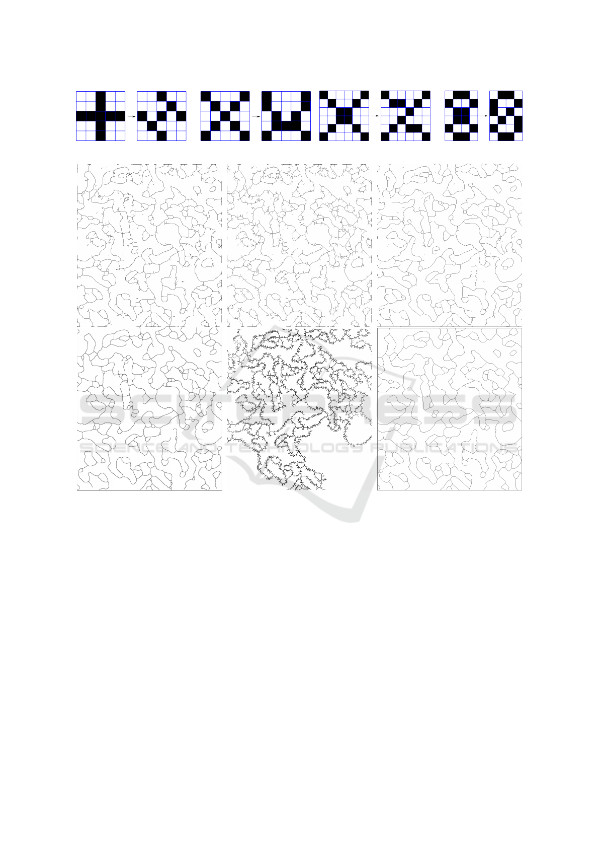
Figure 15: Resolving 2 × 2 black blocks and black pixels with 4 neighbors while preserving the local connectivity.
Figure 16: Output skeletons from past algorithms on the input image in Figure 1 from left to right: (Zhang and Suen,
1984), (Guo and Hall, 1989), (Arganda-Carreras et al., 2010), (Delgado-Friedrichs et al., 2014), (Kamani et al., 2018), ours.
tensity over the mesh, because polygonal edges are
expected to pass through darkest pixels. In addition
to the average intensity, Table 1 includes the number
of components, because a final skeleton should have
one huge component and very few small ones.
The last column in Table 1 counts the total num-
ber of vertices including degree 2 vertices (bends
of polygonal lines). The straightening of polygonal
edges in Stage 3 substantially reduces these degree 2
vertices while the average intensity is only slightly in-
creased to 130.2 and remained smaller than for all
other past algorithms. If we remove small compo-
nents in outputs of (Zhang and Suen, 1984), (Guo and
Hall, 1989) so that their average numbers 177 and 112
of components drop, there will be hundreds (of 433
and 954 on average) degree 1 vertices in Figure 16.
In addition to Table 1, starting from 10 our outputs
on real images, we have generated 625 times more
synthetic ground truth images as follows:
• increased the thickness of skeletons by scaling each
black pixel by a factor k = 1,2,3,4,5.
• applied Gaussian blur for kernel sizes 3,5,7,9,11;
• added Gaussian noise with variances 1,2, 3, 4, 5;
• made 5%,10%,15%,20%,25% random pixels black.
Since (Arganda-Carreras et al., 2010) and
(Delgado-Friedrichs et al., 2014) don’t run for many
images, Table 2 compares our meshes with the
OpenCV algorithms (Zhang and Suen, 1984), (Guo
and Hall, 1989) over 6250 synthetic images.
Pixels in the ground truth and output skeletons are
considered close if they are in 3 × 3 neighborhoods of
each other. The true positives (TP or hits) are pixels in
the output close to ground truth. False positives (TP
or false alarms) are the pixels in the output that are
Polygonal Meshes of Highly Noisy Images based on a New Symmetric Thinning Algorithm with Theoretical Guarantees
143

Table 1: Objective comparison of 6 thinning algorithms (with variations) on more than 100 highly noisy real images.
algorithms / quality measures average intensity connected components deg 1 vertices all vertices
Ground truth 123.7 3 0 819
(Zhang and Suen, 1984): original
Otsu thresholding
135.3 956 1,577 13,927
(Zhang and Suen, 1984): threshold-
ing from section 3
137.6 177 433 30,525
(Guo and Hall, 1989): original Otsu
thresholding
135.7 966 2,417 12,129
(Guo and Hall, 1989): thresholding
from section 3
130.8 112 954 29,927
(Kamani et al., 2018): original Otsu
thresholding
156.7 5 2,653 25,364
(Kamani et al., 2018): thresholding
from section 3
161.3 5 451 61,355
ImageJ (Arganda-Carreras et al.,
2010)
139.2 52 268 30,462
Morse-Smale (Delgado-Friedrichs
et al., 2014)
162.4 3 34 27,612
section 4: without symmetry 145.4 3 0 28,563
section 5: with symmetry 126.7 3 0 23,449
our output after straightening 130.2 3 0 824
Table 2: Accuracy over 6250 synthetic ground truths.
algorithms precision recall F
1
score
Zhang-Suen
(Zhang and
Suen, 1984)
0.068 0.862 0.126
Guo-Hall (Guo
and Hall, 1989)
0.072 0.859 0.133
our method 0.933 0.963 0.948
not close to the ground truth. The false negatives (FN
or misses) are the pixels in the ground truth that are
not close to the output. The accuracy measures in Ta-
ble 2 are precision =
T P
T P + FP
, recall =
T P
T P + FN
and F
1
score = 2
precision × recall
precision + recall
.
The complexity of the algorithm is linear in the
number of pixels, because all steps in sections 3-5 in-
volve small neighborhoods of pixels. The time is less
than 1 sec per image on a laptop with 16GB RAM.
7 DISCUSSION AND
CONCLUSIONS
According to Table 1, the Morse-Smale complex
(Delgado-Friedrichs et al., 2014) is closest to our
vortex mesh in the total number of components and
degree 1 vertices, but has the worst average inten-
sity. The thinning algorithms (Zhang and Suen,
1984), (Guo and Hall, 1989) offered by OpenCV
produce well-centered skeletons (close to our vortex
meshes), but contain too many small components and
degree 1 vertices that are not filtered out. The new
thresholding in section 3 makes these skeletons bet-
ter connected. The performance of AnalyzeSkeleton
(Arganda-Carreras et al., 2010) is roughly between
the Morse-Smale and OpenCV skeletons.
The deep learning papers (Asghari and Jalali,
2015), (Shen et al., 2017) provided their implemen-
tations and trained models. Since our images were
not in their training data, these algorithms performed
poorly on microscopic images because of the inten-
sity variations and noise. An extended version will
include these outputs on images similar to Figure 1.
• The new erosion algorithm in section 4 guarantees
a 1-pixel wide skeleton with a correct homotopy type
(stronger than a graph connectivity) by Theorems 6
and 8. The erosion rules are simpler than those in
(Zhang and Suen, 1984) and (Guo and Hall, 1989).
• The first 6 rows of Table 1 show that the new adap-
tive thresholding in section 3 improves the continuity
of past skeletons by reducing degree 1 vertices.
• The new symmetric thinning in section 5 outper-
forms the past thinning by reducing the average in-
tensity over the mesh to 126.7, which goes up only
slightly after straightening polygonal lines.
• Tables 1, 2 and Figures 17, 18 show that our mesh
is robust under high noise and has better accuracy in
comparison with several past algorithms on more than
100 real and 6250 ground truth images.
VISAPP 2020 - 15th International Conference on Computer Vision Theory and Applications
144
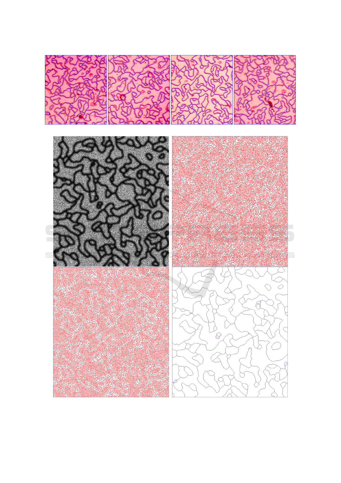
Figure 17: Our final polygonal meshes on more challenging microscopic images with high noise.
Figure 18: 1st: one of 6250 synthetic images with noise over a ground truth skeleton (easy to skeletonize for humans), 2nd:
(Zhang and Suen, 1984), 3rd: (Guo and Hall, 1989), 4th: our output. True Positives are black. False Positives are red. False
Negatives are blue. The OpenCV algorithms (Zhang and Suen, 1984), (Guo and Hall, 1989) output too many false positives.
Polygonal Meshes of Highly Noisy Images based on a New Symmetric Thinning Algorithm with Theoretical Guarantees
145

REFERENCES
Arganda-Carreras, I., Fern
´
andez-Gonz
´
alez, R., Mu
˜
noz-
Barrutia, A., and Ortiz-De-Solorzano, C. (2010). 3d
reconstruction of histological sections: application to
mammary gland tissue. Microscopy Res. & Tech.,
73:1019–1029.
Asghari, M. H. and Jalali, B. (2015). Edge detection in dig-
ital images using dispersive phase stretch transform.
International journal of biomedical imaging.
Bernard, T. M. and Manzanera, A. (1999). Improved low
complexity fully parallel thinning algorithm. In Proc.
Image Analysis and Processing, pages 215–220.
Bernsen, J. (1986). Dynamic thresholding of gray-level im-
ages. In Proc. Intern. Conf. Pattern Recognition.
Canny, J. (1986). A computational approach to edge detec-
tion. Transactions PAMI, 6:679–698.
Delgado-Friedrichs, O., Robins, V., and Sheppard, A.
(2014). Skeletonization and partitioning of digital im-
ages using discrete morse theory. Trans. Pattern Anal-
ysis and Machine Intelligence, 37(3):654–666.
Douglas, D. and Peucker, T. (1973). Algorithms for the
reduction of the number of points required to repre-
sent a digitized line or its caricature. Cartographica,
10(2):112–122.
Guo, Z. and Hall, R. W. (1989). Parallel thinning with two-
subiteration algorithms. Comm. ACM, 32(3):359–373.
Kalisnik, S., Kurlin, V., and Lesnik, D. (2019). A higher-
dimensional homologically persistent skeleton. Ad-
vances in Applied Mathematics, 102:113–142.
Kamani, M., Farhat, F., Wistar, S., and Wang, J. (2018).
Skeleton matching with applications in severe weather
detection. Appl. Soft Computing, 70:1154–1166.
Kurlin, V. (2014a). Auto-completion of contours in
sketches, maps and sparse 2d images based on topo-
logical persistence. In Proceedings of CTIC: Compu-
tational Topology in Image Context, pages 594–601.
Kurlin, V. (2014b). A fast and robust algorithm to count
topologically persistent holes in noisy clouds. In Proc.
Computer Vision Pattern Recogn., pages 1458–1463.
Kurlin, V. (2015a). A homologically persistent skeleton is
a fast and robust descriptor of interest points in 2d im-
ages. In Proceedings of CAIP, pages 606–617.
Kurlin, V. (2015b). A one-dimensional homologically per-
sistent skeleton of an unstructured point cloud. In
Comp. Graphics Forum, volume 34, pages 253–262.
Kurlin, V. (2016). A fast persistence-based segmentation
of noisy 2d clouds with provable guarantees. Pattern
Recognition Letters, 83:3–12.
Lin, S.-Z., Wang, X., Kamiya, Y., Chern, G.-W., Fan, F.,
Fan, D., Casas, B., Liu, Y., Kiryukhin, V., Zurek,
W. H., and Cheong, S.-W. (2014). Topological de-
fects as relics of emergent continuous symmetry and
higgs condensation of disorder in ferroelectrics. Na-
ture Physics, 10(12):970.
Niblack, W. (1985). An introduction to digital image pro-
cessing. Strandberg Publishing Company.
Otsu, N. (1979). A threshold selection method from gray-
level histograms. IEEE transactions on systems, man,
and cybernetics, 9(1):62–66.
Panichev, O. and Voloshyna, A. (2019). U-net based con-
volutional neural network for skeleton extraction. In
Proceedings of the CVPR workshops.
Phansalkar, N., More, S., Sabale, A., and Joshi, M. (2011).
Adaptive local thresholding for detection of nuclei in
diversity stained cytology images. In Intern. Conf.
Comm. and Signal Processing, pages 218–220.
Saha, P. K., Borgefors, G., and di Baja, G. S. (2016). A
survey on skeletonization algorithms and their appli-
cations. Pattern Recognition Letters, 76:3–12.
Sauvola, J. and Pietik
¨
ainen, M. (2000). Adaptive document
image binarization. Pattern Recogn., 33(2):225–236.
Shen, W., Zhao, K., Jiang, Y., Wang, Y., Bai, X., and Yuille,
A. (2017). Deepskeleton: Learning multi-task scale-
associated deep side outputs for object skeleton ex-
traction in natural images. IEEE Transactions on Im-
age Processing, 26(11):5298–5311.
Smith, P. and Kurlin, V. (2019). Skeletonisation algorithms
with theoretical guarantees for unorganised point
clouds with high levels of noise. arXiv:1901.03319.
Soille, P. (2013). Morphological image analysis: principles
and applications. Springer Science & Business.
Soille, P. and Vincent, L. (1990). Determining watersheds
in digital pictures via flooding simulations. In Visual
Comm. Image Proc., volume 1360, pages 240–250.
Wang, Y., Xu, Y., Tsogkas, S., Bai, X., Dickinson, S., and
Siddiqi, K. (2018). Deepflux for skeletons in the wild.
arXiv:1811.12608.
Zhang, T. and Suen, C. Y. (1984). A fast parallel algorithm
for thinning digital patterns. Communications of the
ACM, 27(3):236–239.
VISAPP 2020 - 15th International Conference on Computer Vision Theory and Applications
146
