3D Object Detection from LiDAR Data using Distance Dependent

Feature Extraction

Guus Engels

1 a

, Nerea Aranjuelo

1 b

, Ignacio Arganda-Carreras

2,3,4 c

, Marcos Nieto

1 d

and Oihana Otaegui

1 e

Vicomtech Foundation, Basque Research and Technology Alliance (BRTA), Mikeletegi 57, San Sebastian, Spain

Basque Country University (UPV/EHU), San Sebastian, Spain

Ikerbasque, Basque Foundation for Science, Bilbao, Spain

Donostia International Physics Center (DIPC), San Sebastian, Spain

Keywords:

LiDAR, 3D Object Detection, Feature Extraction, Point Cloud.

Abstract:

This paper presents a new approach to 3D object detection that leverages the properties of the data obtained

by a LiDAR sensor. State-of-the-art detectors use neural network architectures based on assumptions valid for

camera images. However, point clouds obtained from LiDAR data are fundamentally different. Most detectors

use shared ﬁlter kernels to extract features which do not take into account the range dependent nature of the

point cloud features. To show this, different detectors are trained on two splits of the KITTI dataset: close

range (points up to 25 meters from LiDAR) and long-range. Top view images are generated from point clouds

as input for the networks. Combined results outperform the baseline network trained on the full dataset with a

single backbone. Additional research compares the effect of using different input features when converting the

point cloud to image. The results indicate that the network focuses on the shape and structure of the objects,

rather than exact values of the input. This work proposes an improvement for 3D object detectors by taking

into account the properties of LiDAR point clouds over distance. Results show that training separate networks

for close-range and long-range objects boosts performance for all KITTI benchmark difﬁculties.

1 INTRODUCTION

”LiDAR is a fool’s errand and anyone relying on Li-

DAR is doomed.” - Elon Musk, CEO of Tesla. The

CEO of Tesla, a company that puts tremendous ef-

fort in the development of autonomous vehicles does

not see value in using the LiDAR sensor, but a vast

number of researchers and companies disagree and

have shown that including LiDAR in their perception

pipeline can be beneﬁcial for advanced scene under-

standing.

LiDAR is an abbreviation for light detection and

ranging. It is a sensor that uses laser light to mea-

sure the distance to objects and their reﬂectiveness.

It sends out beams of light that diverge over the dis-

tance and reﬂect if an object is hit. It has proven to be

https://orcid.org/0000-0002-4575-4872

https://orcid.org/0000-0002-7853-6708

https://orcid.org/0000-0003-0229-5722

https://orcid.org/0000-0001-9879-0992

https://orcid.org/0000-0001-6069-8787

useful for many applications in areas such as archae-

ology and geology. However, there are some down-

sides that prohibit the adoption of widespread use for

autonomous driving. Currently, LiDAR is an expen-

sive, computationally demanding sensor that requires

some revision of the car’s layout. Cameras are a rich

source of information that are very cheap in compar-

ison. Nonetheless, there are situations where cam-

eras struggle and LiDAR can be of signiﬁcant help.

Driving in low light conditions is challenging for a

camera, but does not make a difference for LiDAR

because it does not depend on external light sources.

Overall, the future of LiDAR and its role in a future

autonomous vehicle is unclear, but it does have very

valuable properties that can play an important role in

autonomous driving and make its research decisive.

For self-driving vehicles it is of the utmost im-

portance to be aware of its surroundings. Therefore,

objects have to be located in the 3D space around

the ego vehicle, which requires using sensors such

as LiDAR to capture the surrounding information.

Research into 3D object detection and LiDAR have

Engels, G., Aranjuelo, N., Arganda-Carreras, I., Nieto, M. and Otaegui, O.

3D Object Detection from LiDAR Data using Distance Dependent Feature Extraction.

DOI: 10.5220/0009330402890300

In Proceedings of the 6th International Conference on Vehicle Technology and Intelligent Transport Systems (VEHITS 2020), pages 289-300

ISBN: 978-989-758-419-0

289

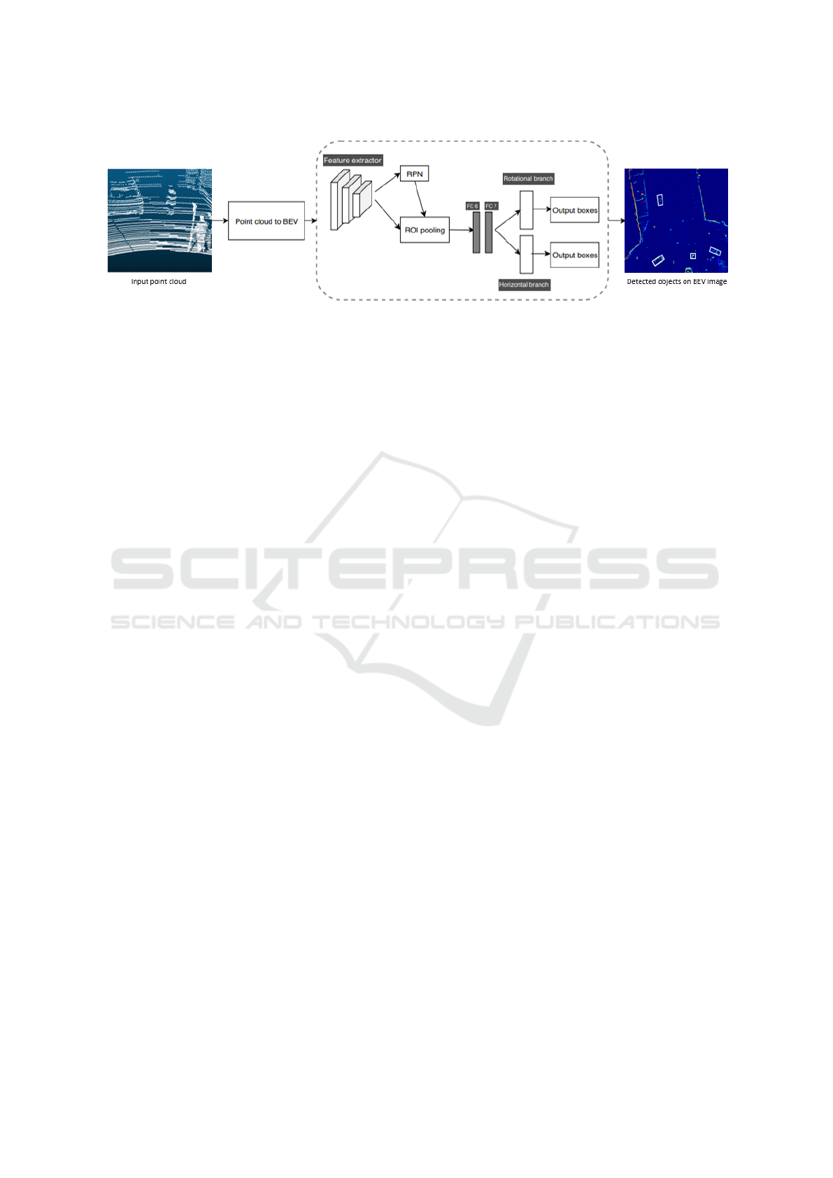
Figure 1: Proposed pipeline for 3D object detection using point clouds as input. In this method, point clouds are converted

to bird’s eye view (BEV) images in the ”point cloud to BEV” stage. The point cloud is compressed to an image according

to one of four conﬁgurations explained in the Methods section. The architecture inside the dotted lines is a Faster R-CNN

architecture with an additional rotation branch that makes it possible to output rotated bounding boxes. RPN stands for region

proposal network, which searches for regions of interest for the head-network that tries to classify and regress bounding boxes

around these objects. ROI pooling converts different sized regions of interest to a common 7 × 7 so it can be handled by two

fully connected layers called FC6 and FC7. The output of these layers are send to the last branches that predict either rotated

or horizontal bounding boxes with a class label.

gone hand in hand. The most inﬂuential dataset for

3D object detection for autonomous applications has

been the KITTI dataset (Geiger et al., 2013). It hosts

leaderboards where different methods are compared.

The growing interest in 3D object detection can be

observed from these leaderboards, where the state of

the art gets replaced quickly by newer architectures.

The best performing network in 2018, Pixor (Yang

et al., 2019a), only just falls in the top 100 as of Octo-

ber 2019. All detectors on the leaderboards, used for

3D object detection are inﬂuenced in varying degrees

by 2D detectors. It is obvious that the advances in

2D object detection can be of big help for 3D object

detection. However, 2D object detection is done on

images, a very different data type compared to point

cloud data. The LiDAR beams diverge, which causes

objects placed farther away to be represented with less

points than the exact same object nearby. This is very

different compared to images, where the object be-

comes smaller when it is farther away, but the under-

lying features and its representation are still the same.

The effect of this has not yet received much attention

in the literature.

In this paper, differences between image and point

cloud data are researched. A new pipeline is pro-

posed that learns different feature extractors for ob-

jects that are close by and far away. This is necessary

because features in these two ranges are very differ-

ent, and one shared feature extractor would perform

sub-optimally in both ranges. Furthermore, visualiza-

tion of the changing features over the distance is pro-

vided. Previous works like ZFnet (Zeiler and Fergus,

2013) were not only able to increase performance, but

also showed the importance of understanding how the

network operates. Inspired by this we focus on how

point cloud input data is different from image input

data to have a better understanding of the limitations

of using 2D CNNs on point clouds. In addition we

show how to alter the detection pipeline to exploit

these differences.

To summarize, the contributions of this paper are

the following:

• We provide an analysis into the effects of different

input features on the detection performance.

• We show the inﬂuence of the changing represen-

tation over distance and how it affects the under-

lying features of the objects on the car class.

• We propose a new detection pipeline that is able

to learn different feature extractors for close-by

objects and far-away objects.

2 RELATED WORK

3D object detection has been tackled with many dif-

ferent approaches. The ﬁrst networks were heavily

inﬂuenced by 2D detectors. They converted point

clouds to top view images, which made it possible

to use conventional 2D detectors. A variety of input

features and conversion methods were used. Many of

these detectors have been later on improved by adding

more information from other sensors or maps.

Currently, most of the best performing architec-

tures use methods that directly process the point cloud

data (Shi et al., 2019; Yang et al., 2019b). They do

not require handcrafted features or conversion to im-

ages like the previous methods did. As of late, new

datasets have become public and will push the ﬁeld of

3D object detection further forward.

VEHITS 2020 - 6th International Conference on Vehicle Technology and Intelligent Transport Systems

290

2.1 2D CNN Approaches

Many early and current 3D object detectors are ad-

justed 2D object detectors such as Faster R-CNN (Ren

et al., 2015) and YOLO (Redmon et al., 2015). In

particular, ResNet (He et al., 2015) is often used as

backbone network for feature extraction. In order to

detect 3D objects with 2D detectors, point clouds are

compressed to image data. Two common representa-

tions are (i) a front view approach like in LaserNet

(Meyer et al., 2019) and (ii) a bird’s eye view (BEV)

approach where point cloud data are compressed in

the height dimension (Beltr

an et al., 2018) . Some

methods only use three input channels to keep the in-

put exactly the same as for 2D detectors. Other meth-

ods use more height channels to save more impor-

tant height information of the point cloud (Yang et al.,

2019a; Chen et al., 2017). Which features are impor-

tant to retain has been researched before but is still an

open research topic. The BEV has proven to be such

a powerful representation that methods using camera

data convert their data to a BEV to perform well on

3D object detection tasks (Wang et al., 2018). How

the conversion from point cloud to BEV is performed

will be explained in the Methods section.

2.2 Multimodal Approaches

A modern autonomous vehicle will have more than

just a LiDAR sensor. This is why many methods use

a multimodal approach that combines LiDAR with

camera sensors (Chen et al., 2017; Liang et al., 2019;

Ku et al., 2018; Qi et al., 2017). Other methods fuse

the data at different stages in the network. MTMS

(Liang et al., 2019) uses an earlier fusion method,

whereas M3VD (Chen et al., 2017) uses a deep fu-

sion method. Besides different sensors, map infor-

mation can also be employed to improve performance

(Yang et al., 2018a). Some approaches track objects

over frames (Luo et al., 2018; Weng and Kitani, 2019)

which boosts performance, especially for objects with

only a small number of LiDAR points and partially

occluded objects in a sequence.

2.3 Detection Directly on the Point

Cloud

A major shift in 3D object detection came when net-

works started to extract features directly from the

point cloud data. Voxelnet (Zhou and Tuzel, 2017)

introduced the VFE layer, which computed 3D fea-

tures from a set of points in the point cloud and stores

the extracted value in a voxel, containing the value

of a volume in 3D space, similar to what a pixel

does for 2D space. A second inﬂuential network that

works directly with the point cloud data is PointNet

(Qi et al., 2016). It processes directly on the un-

ordered point cloud and is invariant to transforma-

tions, such as translations and rotations. These two

methods are the foundation of many architectures in

the top 50 on the KITTI leaderboards. Pointpillars

(Lang et al., 2018) uses PointNet to extract features

and then transform it to a BEV representation to apply

a detector with a FPN inspired backbone (Lin et al.,

2016). Other networks use this approach and focus on

the orientation (Yan et al., 2018) or try bottom up an-

chor generation (Shi et al., 2018; Yang et al., 2018c).

2.4 Datasets

The KITTI dataset (Geiger et al., 2013) has been one

of the most widely used datasets for 3D object detec-

tion for autonomous driving so far. It is a large scale

dataset that contains annotations in the front camera

ﬁeld of view for camera and LiDAR data. There

are three main classes, namely, cars, pedestrians and

cyclists. However, the car class contains more than

half of all objects (Geiger et al., 2013). As of late,

many new datasets have emerged. Most notable are

NuScenes (Caesar et al., 2019) and the H3D dataset,

of Honda (Patil et al., 2019). They are much larger

datasets, 360 degrees annotated and contain 1 million

and 1.4 million bounding boxes (respectively) com-

pared to 200k annotations in KITTI. The NuScenes

dataset was created with a 32-channel LiDAR, in

comparison to the KITTI and H3D dataset which

were both created with a 64-channel LiDAR. Sen-

sors with more channels are able to produce denser,

more complete 3D maps. The beam divergence will

be larger when there are less channels and will make

it more difﬁcult to detect objects far away.

3 METHODS

In order to apply 3D object detection on LiDAR and

perform the different tests mentioned in the Introduc-

tion, a 3D object detection algorithm is implemented

according to the structure in Figure 1. The point cloud

is converted to images, which can then be used by

a Faster R-CNN detection network. This network is

used to evaluate the effect of different input features

on the performance and to create an architecture that

uses different kernel weights for different regions of

the LiDAR point cloud.

3D Object Detection from LiDAR Data using Distance Dependent Feature Extraction

291

3.1 Network

3.1.1 Architecture

The architecture of the full baseline network is dis-

played in Figure 1. The full architecture has a point

cloud as input and outputs horizontal and rotational

bounding boxes. A Faster R-CNN (Ren et al., 2015)

with a rotation regression branch in the head network

is used. The backbone network is ResNet-50 (He

et al., 2015) of which only the ﬁrst three blocks are

used for the RPN network. Faster R-CNN is designed

for camera images where objects can have all kinds of

shapes. In a BEV image of LiDAR data all objects are

relatively small in comparison. To make sure that the

feature map is not downsampled in size too quickly,

the stride of the ﬁrst ResNet block is adjusted from 2

to 1. This causes the output feature map to be four

times as big, which means that less spatial informa-

tion is lost. The object size in a BEV image is di-

rectly proportional to the physical size of that object.

This allows for tailoring the anchor boxes exactly to

the object size to serve as good priors. When cars are

rotated these anchor boxes will not ﬁt accurately to

the objects. To account for this, different orientations

of the anchor boxes are considered similarly to (Yang

et al., 2018b; Simon et al., 2019). In total, sixteen dif-

ferent orientations in the anchor boxes are used. The

head network is slightly different from Faster-RCNN

because it contains an additional rotation head (Jiang

et al., 2017). Region proposals from the RPN network

and the output feature map of the RPN network are the

inputs of the head network. Region of interest pooling

(ROI) outputs 7 × 7 × 1024 feature maps for each ob-

ject proposal that are fed to two fully connected lay-

ers with 1024 parameters. These layers output four

bounding box variables for non rotated objects, more

speciﬁcally, the center of the box coordinates (x, y)

and the dimensions (h, w). The rotated boxes have an

additional parameter, θ, for the rotation angle of the

bounding box. Each box has a class conﬁdence score.

The class with the highest score is the most likely for

this bounding box and it is used as output.

3.1.2 Point Cloud to BEV Image

Feature extractors such as ResNet are designed for

RGB images. Using this exact architecture requires

reshaping the point cloud input to a three channel im-

age. A common approach consists of compressing

the point cloud into a BEV image where the height

dimension is represented by three channels. Which

information to keep remains an open problem. In the

past, it was shown that the reﬂectiveness, or inten-

sity value, did not contribute much when there was

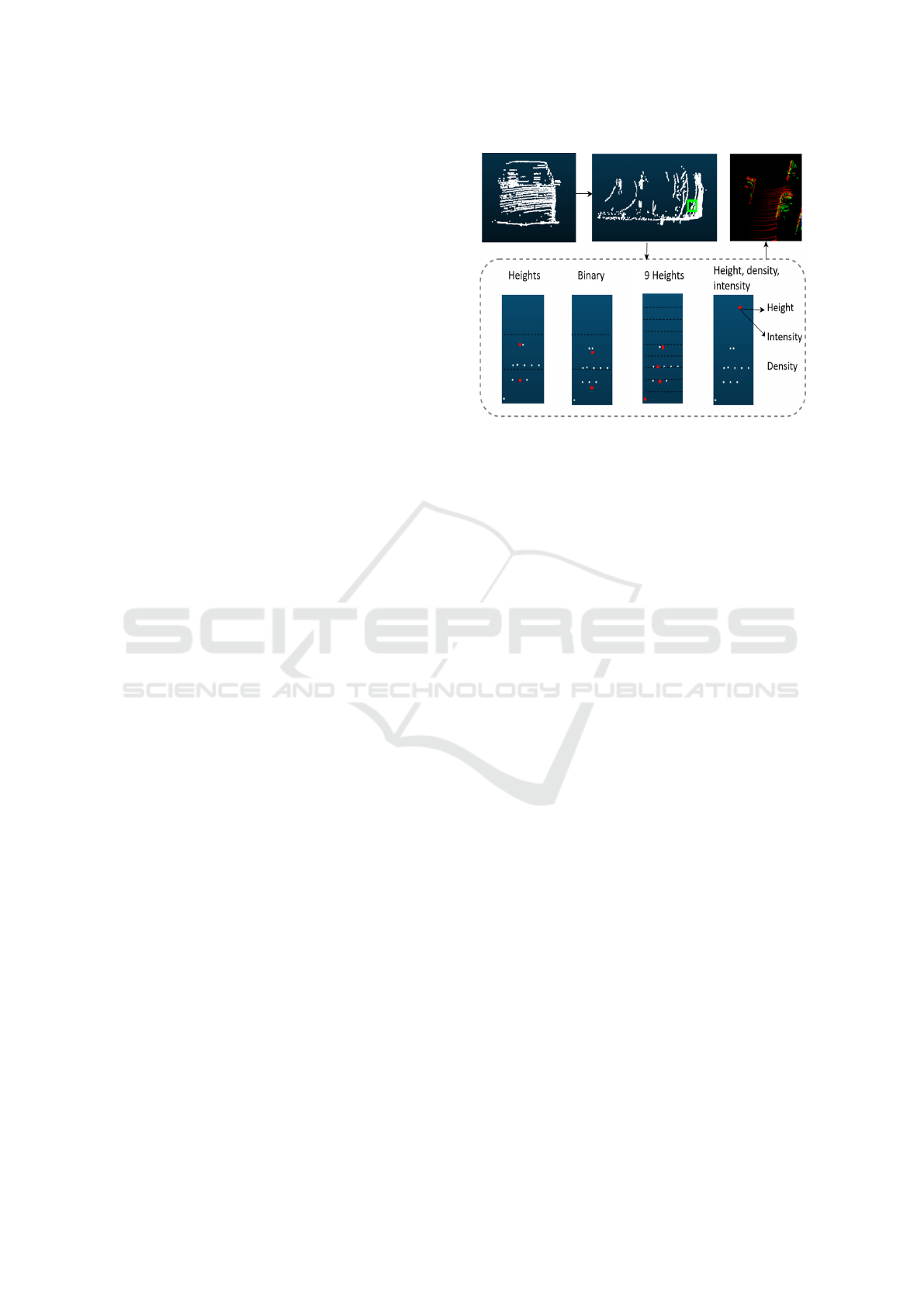
Figure 2: Point cloud conversion to bird’s eye view (BEV)

representation. This research uses four different possi-

ble conﬁgurations that are visualized in the bottom dotted

block. In the complete pipeline only one of these will be

used for each test.

maximum height information available (Beltr

an et al.,

2018). Pixor (Yang et al., 2019a) and MV3D (Chen

et al., 2017) use multiple height maps to retain more

height information. Instead of only storing 3 chan-

nels, as it would be the case in a regular 2D detec-

tor, they have an architecture that can handle inputs

of more than 3 channels. To test the effect of dif-

ferent features, the inputs are pre-processed in four

different input conﬁgurations. For all methods there

are some shared steps. Firstly, a 3D space of 0m

to 70m in longitudinal range, −35m to 35m in lat-

eral range and −1.73m to 1.27m in the height dimen-

sion is deﬁned. The LiDAR in the KITTI setup is

located 1.73m off the ground, so −1.73m is where

the road is. All points that fall outside of this box

are not taken into account. For three of the four meth-

ods, 700 ×700×3 pixel images are considered, which

means that every 0.1 × 0.1 × 3m cube represents one

pixel. The last method uses more channels and is of

size 700 × 700 × 9. The exact speciﬁcations of the

channels are as follows:

Max Height Voxels: the cube can be divided in three

voxels with each 0.1m × 0.1m × 1m dimensions. The

ﬁrst channel will have the height value of the highest

point from −1.73m to −0.73m range. The second

channel will have the highest value from −0.73m to

0.23m and the third one from 0.23m to 1.23m. An ad-

vantage of this method is that automatically a form of

ground removal takes place. The points very close to

the road are often not of much importance for the ob-

jects on the road. In addition, the highest points of an

object are in many cases what distinguishes them, and

therefore often the most important feature (Beltr

et al., 2018).

VEHITS 2020 - 6th International Conference on Vehicle Technology and Intelligent Transport Systems

292

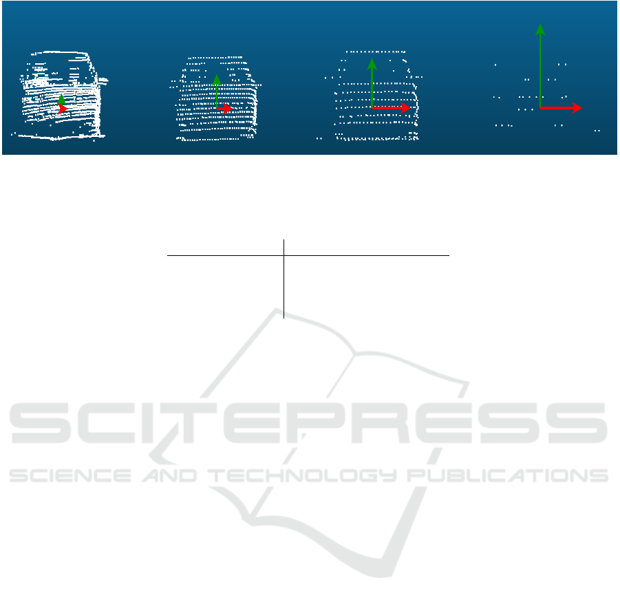
Figure 3: Representation of four cars at different ranges detected with a 64 channel LiDAR. The green arrow indicates the

vertical distance between four adjacent points and the red arrow indicates the horizontal distance between four adjacent points.

The distance of four points instead of the distance between adjacent points is used for visualization purposes.

Table 1: Statistics of the 4 cars, ordered from left to right.

Car number 1 2 3 4

distance [m] 7.6 16.0 24.4 43.0

vert spacing [cm] 4 9 13 22

hor spacing [cm] 2 5 8 13

amount of points 1797 627 226 25

Binary: for every voxel it is checked if there is at

least one LiDAR point present. If this is the case, this

channel gets the value 100, if not it gets the value 0.

The value 100 is chosen instead of 1 to make sure the

values have the same order of magnitude as the pre-

trained Imagenet (Deng et al., 2009) weigths. This

approach is an important indicator of how the network

handles the speciﬁc point cloud values. Consequently,

it is a baseline test to see if other features add value.

Multichannel Max Height Voxels: the input of only

three channels might not be enough since it means

that many of the original point cloud information is

lost. Using more height will provide the network with

more of the original information and should improve

the scores as was done in (Chen et al., 2017; Yang

et al., 2019a). Nine height maps are used as input to

the ResNet backbone instead of the three maps used

in the max height approach. To make sure that this

input is compatible with the ResNet feature extractor,

the pre-trained weights are duplicated three times and

stacked.

Height Intensity Density: instead of picking a subset

of the points from the point cloud, it is also possible

to compute features that could be interesting and feed

them to the network. This conﬁguration has been used

in Birdnet (Beltr

an et al., 2018) before.

A visualization of how all the features are ex-

tracted is displayed in Figure 2. This stage represents

what happens in the ”Pointcloud to BEV” block in

Figure 1.

3.2 Loss Function

Faster R-CNN is a two-stage detector for which the

total loss is a combination of the losses of the individ-

ual stages. The losses of the ﬁrst stage are similar to

the original Faster R-CNN paper, but do not have the

logarithmic scaling factors. There are regression tar-

gets that describe the absolute difference between the

ground truth and the network prediction for the center

points (x, y) and the dimensions (h, w) of the object:

∆x

= x

− x

(1)

∆y

= y

− y

(2)

∆h = h − h

(3)

∆w = w − w

(4)

where x

,h, w are predictions from the network

and x

are the ground truth targets which

the network aims to predict. The classiﬁcation loss is

a softmax cross-entropy between the background and

foreground classes. Together they form the RPN loss.

The horizontal branch of the head network uses

the exact same regression targets, but should now con-

sider multiple, instead of just background and fore-

ground classes. In this research, only the car class is

considered so it turns out to be the same as for the

RPN case. The rotational branch of the head network

has an additional regression loss for the rotation as

show in Figure 1. This loss is the absolute difference

between the predicted and ground truth angle in de-

grees:

∆θ = θ − θ

(5)

3D Object Detection from LiDAR Data using Distance Dependent Feature Extraction

293

It is important to note that by introducing rotation

it becomes possible to describe the exact same rotated

bounding box in multiple ways. Consider a bound-

ing box deﬁned by x

, y

, h, w, and θ. If the values

of h and w are swapped and 90 degrees are added to

the angle θ, the same bounding box can be described.

This has to be avoided since a loss larger than zero

would be possible, even though the predict bounding

box ﬁts perfectly. This is avoided by making sure that

the width is always larger than the height. If this is

not the case the height and width are swapped and

90 degrees are added to the rotation to force unique

bounding box conﬁgurations.

Once all regression targets are calculated smooth

L1 loss is used according to the following equation:

L1(x) =

(

0.5x

σ if |x| <

0.5

|x| −

0.5

otherwise

(6)

where σ is a tuning hyperparameter, σ = 3 for the

RPN network and σ = 1 for the head network are

used, which is in line with Faster R-CNN implemen-

tation (Ren et al., 2015).

Combining the classiﬁcation and regression losses

for all branches results in six total losses. A classiﬁ-

cation and regression loss for the RPN, horizontal and

rotational branch. All losses use smooth L1 loss to

calculate the total loss value according to the follow-

ing equation:

Loss = L

rpn,reg

+ L

rpn,class

+ L

head

,reg

+ L

head

,class

+ L

head

,reg

+ L

head

,class

(7)

where L

rpn,reg

is the regression loss of the RPN,

rpn,class

is the classiﬁcation loss of the RPN,

head

,reg

is the regression loss of the horizontal head

network, L

head

,class

is the classiﬁcation loss of the

horizontal head network, L

head

,reg

is the regression

loss of the rotational head network and L

head

,class

the classiﬁcation loss of the rotational head network.

3.3 The Difference of LiDAR Data

The density and distance between points change over

distance in the point clouds. Deep learning architec-

tures are often designed with images in mind where

this is not the case. The section shows how features

change in the LiDAR data and how the network archi-

tecture can be adjusted to account for this.

3.3.1 LiDAR Features

An important reason why convolutional neural net-

works are able to work well with relatively few pa-

rameters compared to classic neural networks, is be-

cause of parameter sharing. It leverages the idea that

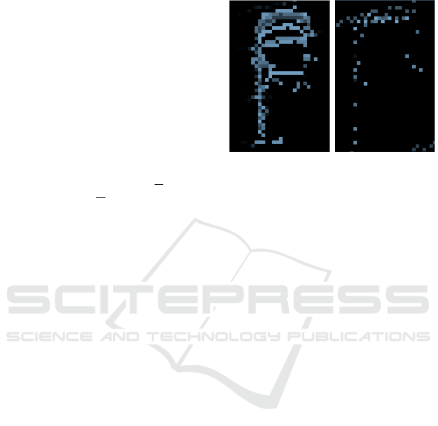
Figure 4: BEV representation of two cars in the same KITTI

frame. The left car is located at 20 meters from the LiDAR

and the right car is located 53 meters from the LiDAR. It can

be seen that the amount of points decreases over distance

and gaps start appearing between adjacent pixels.

important features are the same across the whole im-

age and a single ﬁlter can be used at every position

(Goodfellow et al., 2016). This is a valid assump-

tion for rectilinear images but not for LiDAR data.

The representation of an object is different 5m from

the sensor compared to 20m from the sensor. The

amount of points reduces and the distance between

different points increases. Figure 3 shows how the

representation of a car changes over distance. The

amount of points drastically decreases, for an object

of the same class and similar size, while the distance

between points increases.

The sparsity and divergence of the beams over

time can also be observed in BEV images. Figure 4

shows the gaps that appear in the side of a car. This

is not because there is not part of the car at that pixel

but because the beams have diverged so far that it is

simply not possible to cover all pixels with the beams.

The farther away from the LiDAR, the larger the gaps.

Note that these gaps in longitudinal and lateral dimen-

sion are much smaller compared to the divergence in

the height dimension. The rapid divergence in the

height dimension makes it difﬁcult to detect objects

that only cover a small area such as pedestrians. The

green arrow in Figure 3 represents the height dimen-

sion and shows a bigger distance than the red arrow

which relates to the longitudinal and lateral dimen-

sions. This is conﬁrmed by looking at the speciﬁca-

tions of the LiDAR used for the KITTI dataset, which

state that the angular resolution in longitudinal and

lateral range is 0.09 degrees and the vertical reso-

lution is 0.4 degrees (LiDAR, ). The fourth car in

Figure 3 is barely distinguishable at a distance of 43

meters. The BEV range is 70 by 70 meters so con-

sidering that range, 43 meters is not even near the

VEHITS 2020 - 6th International Conference on Vehicle Technology and Intelligent Transport Systems

294

edge of where cars should be detected for the KITTI

evaluation. The difﬁculties for far-away objects in the

KITTI dataset were quite recently addressed by Wang

et al. (Wang et al., 2019). They used adaptive lay-

ers to enhance the performance on distant objects and

were able to improve SECOND (Yan et al., 2018) and

VoxelNet (Zhou and Tuzel, 2017) with roughly 1.5%

average precision for easy, moderate and hard cate-

gories. While the idea here is similar, our work does

not need an adversarial approach.

3.3.2 Combined Network

With the knowledge that features are not consistent

over the range of the point cloud, the network can be

adjusted accordingly. Multiple instances of the base-

line network are used and trained on different subsets

of the training data. The ﬁrst network is only trained

on the objects that are close by, while an identical

second network is trained on objects far away. The

results of the separate regions are combined and then

compared to a baseline network that is trained on the

full range. To decide if objects should fall in the cate-

gory ”close by” or ”far away” a distance threshold has

to be established. From ﬁgure 5 it can be seen that a

radial distance from the LiDAR sensor is used.

For the inside range, the point cloud is converted

to a BEV image in the same manner as before, but

now all the pixel values outside this threshold range

are set to zero. This is done similarly for the outside

range but the inside set of pixels is set to zero as dis-

played in Figure 5. The point cloud is converted to

two BEV images. Each one contains part of the point

cloud and part of the objects. If the distance to the

center of an object is smaller than the threshold range

it belongs to the inside network and if it is larger it

belongs to the outside network.

When objects are excluded based on their center,

it could happen that objects are partially cut out of

the image and fed to the network. This should not

occur since it will devalue the training data. To avoid

this, an overlap region is introduced. This region is of

the point cloud is used both for the inside and outside

range networks.

4 IMPLEMENTATION DETAILS

4.1 Network Settings

All tests are done on a Faster R-CNN network with

a rotational branch inspired by (Xue, 2018). A learn-

ing rate of 0.0003 with decay steps at 190k and 230k

with a decay factor of 3 for both steps is applied. The

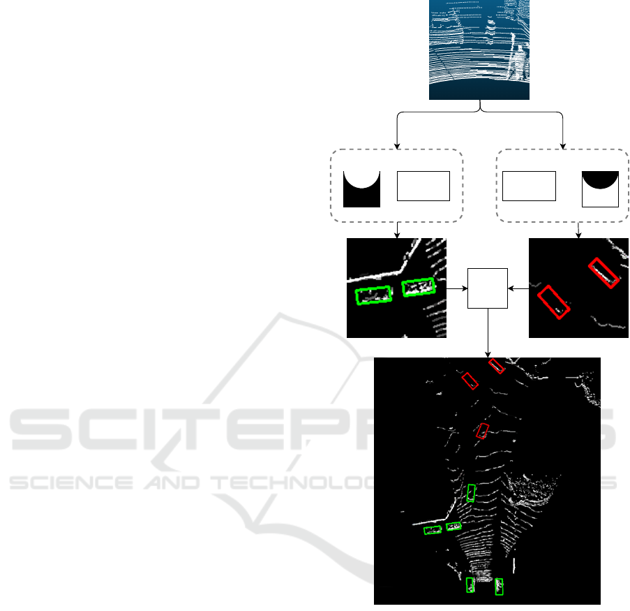
Inside range

network

Outside range

network

Combine

outputs

Figure 5: Pipeline of the combined network architecture.

Inside and outside range network only consider the white

part of the visualized range next to them. These networks

have the exact same conﬁguration and are in line with Fig-

ure 1. The outputs of both networks are combined to form

the ﬁnal output.

dataset, which contains 7481 samples, is split in train-

ing, validation and testing in a 50/25/25 fashion. For

all networks, multiple checkpoints were evaluated and

the one with the best score on the validation set was

picked. The best scores occurred often between 200k

and 250k steps which means that the network were

trained for roughly 50 to 60 epochs. All networks are

trained on a single Nvidia Tesla V100 GPU. Anchors

of 45 × 20 pixels are used to detect cars which is in

line with the average car size.

3D Object Detection from LiDAR Data using Distance Dependent Feature Extraction

295

The network is optimized using stochastic gradi-

ent descent with momentum of 0.9. Weight decay

of 0.0001 is used to prevent overﬁtting. All weights

of the ResNet backbone are pre-trained on ImageNet

(Deng et al., 2009). The underlying data is quite

different from the LiDAR data but we observed fast

convergence for the network. A batch size of 1 is

used with batch normalization applied with a decay

factor of 0.997. Batch normalization is applied but

not trained, the values from the pre-trained ImageNet

weights are used for the batch normalization layer.

Smooth L1 loss is used with thresholds of 3 and 1

for the RPN and head network respectively. The loss

weights for the different components are found em-

pirically. It is important to note that only one class

is considered during training, which makes classiﬁ-

cation easier. Most errors occurred in the box calcu-

lation so the regression loss is twice as high as the

classiﬁcation loss for both RPN and head network

branches.

4.2 Data Pre-processing

Point clouds are converted to one of the four conﬁg-

urations described in the Methods section, displayed

in Figure 2. Every pixel corresponds to 0.1 × 0.1 me-

ter space in the point cloud. All tests are done on the

KITTI dataset where only the ﬁeld of view (FOV) of

the front camera is annotated. All pixel values out-

side this FOV are set to zero which results in a region

of black pixels. Some objects that lay on the border

are sometimes still annotated. To generalize this sit-

uation for all images, only objects that are annotated

and have at least 50% of the surface in the FOV are

taken into account. No augmentations are used for the

ﬁnal models because they did not improve the perfor-

mance of the network.

4.3 Combined Network

The combined network uses the exact same settings

described in the previous sections, but applied to dif-

ferent range. One network is trained on data close to

the LiDAR while the another network is trained on

data far away from the LiDAR. The ﬁnal output is

their combined output for the respective regions. For

the inside range network only boxes with the center

closer than 25m to the LiDAR are taken into account.

With a 5m overlap region between 25m and 30m, to

make sure no labeled objects are cut in half. For the

network that trains on objects that are far away, a 30m

boundary is used where the 25 − 30m region is the

overlap region mentioned before. Figure 5 shows how

the images are combined. The choice of the threshold

Table 2: Results of different input feature conﬁgurations.

Features Easy Moderate Hard

max height 79.5 73.1 66.6

height, intensity, density 79.2 73.1 67.0

binary 79.4 72.9 66.4

multichannel height vox. 76.0 65.8 65.0

for a particular dataset affects the results of the net-

work. We found that 25m was a good threshold since

both regions still contain enough training samples.

For inference a more straight forward division is

used. The KITTI evaluation considers a range of

[−35m, 35m] laterally and [0m, 70m] longitudinally.

We simply divided this region in half to get a close

by and far away range where we evaluate the baseline

and combined network on. All objects in the top half

of the image bounded by [−35m, 35m] laterally and

[0m, 35m] longitudinally will be detected by the in-

side network. The outside network detects objects in

a space bounded by [−35m, 35m] laterally and [35m,

70m]. The results of both networks are then merged

together. The full pipeline is displayed in Figure 5.

5 RESULTS

All results are based on the KITTI benchmark which

calculates average precision (AP) scores for three

different categories, respectively easy, moderate and

hard. AP is an often used object detection metric. In

KITTI, 41 equally spaced recall points are used where

the precision at each point is calculated. Precision is

evaluated at different recall points and combined ac-

cording to the following equation:

kitti

p(r)dr (8)

where r is a set of 41 values linearly spaced be-

tween [0, 1] where each value is a speciﬁc recall value.

The integral of all recall values divided by 41 is the

AP score.

Different true positive thresholds are considered.

The ofﬁcial KITTI has a 70% intersection over union

(IoU) threshold for the car class but we also report

scores for 50% overlap as many other works analyse.

70% percent is quite challenging to achieve with ro-

tational bounding boxes around objects that are often

occluded or contain few points.

5.1 Feature Analysis

Multiple different input features and their impact on

results are tested next. In the methods section, the

VEHITS 2020 - 6th International Conference on Vehicle Technology and Intelligent Transport Systems

296

Table 3: Baseline network compared to the combined network for 50% and 70% IoU threshold. The average precision for the

0-70 meter range is the weighted mean average precision of the 0-35 range and the 35-70 range. The reason for this is that the

conﬁdence scores of the combined network do not match. The conﬁdence scores of the objects far away are too high because

that network has never seen objects close by. This difference in conﬁdence score between the two networks inﬂuences the AP

calculations, so a mean average precision of the two ranges is used.

0-35m range 35-70m range 0-70m range

Method (Threshold) Easy Moderate Hard Easy Moderate Hard Easy Moderate Hard

Baseline (0.7) 78.8 82.0 75.4 - 43.7 37.0 78.5 73.0 66.9

Combined Network (0.7) 81.5 83.4 76.5 - 46.5 42.0 81.2 74.7 68.9

Difference 2.7 1.4 1.1 - 2.8 5.0 2.7 1.7 2.0

Baseline (0.5) 89.3 89.7 89.2 - 60.9 53.0 89.0 82.9 81.2

Combined Network (0.5) 89.8 89.9 89.5 - 75.1 67.7 89.5 86.4 84.7

Difference 0.5 0.2 0.3 - 14.2 14.7 0.5 3.5 3.5

considered four different input conﬁgurations are ex-

plained. Table 2 shows the results on the KITTI

benchmark for the different pre-processing meth-

ods displayed in Figure 2. It can be seen that the

ﬁrst three methods, maximum heights, binary and

height/intensity/density only differ by a small mar-

gin. Only the approach where 9 channels are used

performs signiﬁcantly worse.

Overall the networks seem to learn more the struc-

ture of the objects and not the absolute values stored

in the channels. This does not come as a complete

surprise since a ResNet feature extractor with batch

normalization is used. The information of the abso-

lute values is ”lost” quite quickly in the network be-

cause of the normalization. The ﬁlters in the ﬁrst lay-

ers search more for derivative-based features such as

edges and corners. From that perspective, the differ-

ences are not so big. With that being said, the input

values are still important for the performance of the

network. Solely using intensity has a much worse

performance than only using the max height value

(Beltr

an et al., 2018). Another factor could be the pre-

trained weights. That allows for fast training results

but may limit the overall performance of the network.

This could be a problem especially for the network

with nine channel inputs.

These results highlight a limitation of 2D detec-

tors processing on point clouds and a possible reason

for the gap between them and methods directly us-

ing the point cloud. For LiDAR data these absolute

values are of big importance, since they can give in-

formation about classes directly. An object is very

unlikely to be a car if the highest values are only 1

meter high even though the top view almost perfectly

corresponds. It is possible that methods that use the

point cloud directly are able to leverage this infor-

mation more than 2D detectors. These networks also

use batch normalization but are able to compute more

complete features that help boost their scores. Rely-

ing too heavily on these input values could be danger-

ous when considering different classes, noise, sensor

movement, etc. With the rise of new datasets, it will

hopefully become clear how robust these methods are.

5.2 Range Analysis

Table 3 shows the results of the baseline network and

the combined network on a 70% IoU threshold and a

50% threshold. Easy category is not considered for

35-70m range analysis, due to the lack of signiﬁcant

amount of cars. The combined network outperforms

the baseline network for all categories. The inside and

outside networks are trained on subsets of the total

data and are still able to perform better than the base-

line network. Not sharing the weights results in a bet-

ter performing network, because objects in different

ranges do not have to share the same feature extrac-

tors.

The results of 50% IoU compared to the ones with

70% show that even if the networks are able to detect

the cars, in many cases the precision of the bound-

ing boxes hurts the results signiﬁcantly. Cars that are

closer to the LiDAR contain more points and regress-

ing their boxes is easier in these situations. If only a

50% threshold is used, the evaluation is more forgiv-

ing for errors in rotation because they have the largest

inﬂuence on the overlap. For the 35-70m range the

improvements of the combined network are remark-

able. It seems that the difference in features over the

distance hurts the ability to detect objects, when the

model is trained with full range data. The same hap-

pens with the ability to detect the orientation of the

objects accurately. In automated driving this is impor-

tant since the orientation is key for further processing

steps such as estimating heading angles and applying

tracking.

Figure 6 shows qualitative results of the combined

network. The green boxes are from the inside network

and the red boxes from the outside network. The BEV

image is adjusted for better visualization by smooth-

3D Object Detection from LiDAR Data using Distance Dependent Feature Extraction

297

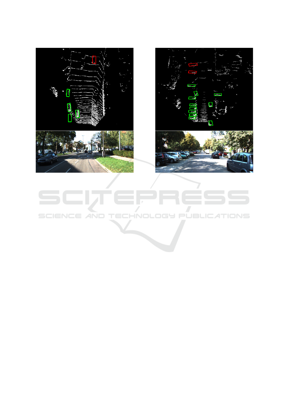
Figure 6: Detection results on KITTI validation set. The upper row in each image is the BEV representation with the detected

cars. The other are the camera images corresponding to those BEVs. Green boxes are estimated by the inside network and

red boxes by the outside network.

ing the images and maximizing the input values. In

the left image, it can be appreciated that the closest

bounding box to the LiDAR is a correct detection, al-

though almost all of the pixels that represent the car

are black. The algorithm is able to detect it correctly

based on the small corner that is still present. The

right ﬁgure shows how the network performs all over

the range.

6 DISCUSSION

A 3D object detection algorithm is implemented and

trained on the KITTI dataset, that outperforms many

recent BEV based networks (Simon et al., 2019;

Beltr

an et al., 2018; Meyer et al., 2019) and gets simi-

lar results to other networks (Yang et al., 2019a; Chen

et al., 2017). This paper shows how convolutional

neural networks used for natural images are based on

assumptions that do not transfer well to point cloud

data. This concept can be used to increase the perfor-

mance of many networks on the KITTI benchmark

whether they are processing BEV images or point

clouds directly as was also shown by (Wang et al.,

2019). Furthermore it looks into the advantages and

limitations of BEV approaches. The main advantage

is robustness since it does not rely on the speciﬁc val-

ues of the object, but mostly on the shape. This could

also be thought as a limitation since these speciﬁc val-

ues could be directly used for classiﬁcation in LiDAR

data. However, these values can vary between LiDAR

models and are more sensitive to possible noise. Data

quantity that needs to be processed is another thing to

take into account, as only an image needs to be pro-

cessed instead of an entire point cloud.

7 CONCLUSIONS

This work provides insights in how LiDAR data dif-

fers from natural images, which features are impor-

tant for detecting cars and how a neural network ar-

chitecture for 3D object detection can be adjusted to

take into account the changing object features over the

distance. The ﬁrst tests check the effect of different

handcrafted input features on the performance. Point

clouds are converted to BEV images that are fed to a

two stage detector. Different input conﬁgurations do

not vary much in performance which can be attributed

to the fact that the ﬁlters look for features such as

edges and do not rely as much on the exact values

in the BEV. These exact values are of more relevance

for LiDAR data compared to camera images because

they can be linked directly to certain classes. This

VEHITS 2020 - 6th International Conference on Vehicle Technology and Intelligent Transport Systems

298

is different from approaches that use the raw point

clouds directly as input and might explain why they

perform overall better on the KITTI benchmark. Nev-

ertheless, relying on those values may be a problem

when dealing with sensor noise or model differences.

With the rise of new datasets, it will hopefully become

clear how robust these methods are compared to BEV

based approaches.

In addition, this work visualizes how the distance

to the sensor inﬂuences the objects representation in

the point cloud. Most convolutional neural network

rely on the assumption that features are consistent

over the full range of the image. This allows for one

ﬁlter to be used to extract features from the entire fea-

ture map. For LiDAR data this is not the case which

is shown by analyzing point clouds and objects at var-

ious distances. This observation is used to change the

detection pipeline and have a separate detector for ob-

jects in the 0-35 meter range and another detector for

objects in the 35-70 meter range. These changes lead

to improvements, most notably of 2.7% AP on the 0-

35 meter range for easy category and 5.0% AP on the

35-70 meter range for hard category, using a 70% IoU

threshold.

REFERENCES

Beltr

an, J., Guindel, C., Moreno, F. M., Cruzado, D.,

Garc

ıa, F., and de la Escalera, A. (2018). Birdnet: a

3d object detection framework from lidar information.

CoRR, abs/1805.01195.

Caesar, H., Bankiti, V., Lang, A. H., Vora, S., Li-

ong, V. E., Xu, Q., Krishnan, A., Pan, Y., Baldan,

G., and Beijbom, O. (2019). nuscenes: A multi-

modal dataset for autonomous driving. arXiv preprint

arXiv:1903.11027.

Chen, X., Ma, H., Wan, J., Li, B., and Xia, T. (2017). Multi-

view 3d object detection network for autonomous

driving. In Proceedings of the IEEE Conference

on Computer Vision and Pattern Recognition, pages

1907–1915.

Deng, J., Dong, W., Socher, R., Li, L.-J., Li, K., and Fei-

Fei, L. (2009). ImageNet: A Large-Scale Hierarchical

Image Database. In CVPR09.

Geiger, A., Lenz, P., Stiller, C., and Urtasun, R. (2013).

Vision meets robotics: The kitti dataset. International

Journal of Robotics Research (IJRR).

Goodfellow, I., Bengio, Y., and Courville, A. (2016). Deep

Learning. The MIT Press.

He, K., Zhang, X., Ren, S., and Sun, J. (2015). Deep

residual learning for image recognition. CoRR,

abs/1512.03385.

Jiang, Y., Zhu, X., Wang, X., Yang, S., Li, W., Wang, H.,

Fu, P., and Luo, Z. (2017). R2CNN: rotational re-

gion CNN for orientation robust scene text detection.

CoRR, abs/1706.09579.

Ku, J., Moziﬁan, M., Lee, J., Harakeh, A., and Waslander,

S. (2018). Joint 3d proposal generation and object de-

tection from view aggregation. IROS.

Lang, A. H., Vora, S., Caesar, H., Zhou, L., Yang, J.,

and Beijbom, O. (2018). Pointpillars: Fast en-

coders for object detection from point clouds. CoRR,

abs/1812.05784.

Liang, M., Yang, B., Chen, Y., Hu, R., and Urtasun, R.

(2019). Multi-task multi-sensor fusion for 3d object

detection. In The IEEE Conference on Computer Vi-

sion and Pattern Recognition (CVPR).

LiDAR, V. Hdl-64 users manual.

Lin, T., Doll

ar, P., Girshick, R. B., He, K., Hariharan, B.,

and Belongie, S. J. (2016). Feature pyramid networks

for object detection. CoRR, abs/1612.03144.

Luo, W., Yang, B., and Urtasun, R. (2018). Fast and furious:

Real time end-to-end 3d detection, tracking and mo-

tion forecasting with a single convolutional net. 2018

IEEE/CVF Conference on Computer Vision and Pat-

tern Recognition, pages 3569–3577.

Meyer, G. P., Laddha, A., Kee, E., Vallespi-Gonzalez, C.,

and Wellington, C. K. (2019). Lasernet: An efﬁcient

probabilistic 3d object detector for autonomous driv-

ing. CoRR, abs/1903.08701.

Patil, A., Malla, S., Gang, H., and Chen, Y. (2019). The

H3D dataset for full-surround 3d multi-object detec-

tion and tracking in crowded urban scenes. CoRR,

abs/1903.01568.

Qi, C. R., Liu, W., Wu, C., Su, H., and Guibas, L. J. (2017).

Frustum pointnets for 3d object detection from RGB-

D data. CoRR, abs/1711.08488.

Qi, C. R., Su, H., Mo, K., and Guibas, L. J. (2016). Pointnet:

Deep learning on point sets for 3d classiﬁcation and

segmentation. CoRR, abs/1612.00593.

Redmon, J., Divvala, S. K., Girshick, R. B., and Farhadi, A.

(2015). You only look once: Uniﬁed, real-time object

detection. CoRR, abs/1506.02640.

Ren, S., He, K., Girshick, R. B., and Sun, J. (2015). Faster

R-CNN: towards real-time object detection with re-

gion proposal networks. CoRR, abs/1506.01497.

Shi, S., Wang, X., and Li, H. (2018). Pointrcnn: 3d object

proposal generation and detection from point cloud.

CoRR, abs/1812.04244.

Shi, S., Wang, Z., Wang, X., and Li, H. (2019). Part-aˆ

2 net: 3d part-aware and aggregation neural network

for object detection from point cloud. arXiv preprint

arXiv:1907.03670.

Simon, M., Amende, K., Kraus, A., Honer, J., S

amann,

T., Kaulbersch, H., Milz, S., and Gross, H.

(2019). Complexer-yolo: Real-time 3d object detec-

tion and tracking on semantic point clouds. CoRR,

abs/1904.07537.

Wang, Y., Chao, W., Garg, D., Hariharan, B., Campbell,

M., and Weinberger, K. Q. (2018). Pseudo-lidar

from visual depth estimation: Bridging the gap in

3d object detection for autonomous driving. CoRR,

abs/1812.07179.

Wang, Z., Ding, S., Li, Y., Zhao, M., Roychowdhury, S.,

Wallin, A., Sapiro, G., and Qiu, Q. (2019). Range

adaptation for 3d object detection in lidar.

3D Object Detection from LiDAR Data using Distance Dependent Feature Extraction

299

Weng, X. and Kitani, K. (2019). A baseline for 3d multi-

object tracking. CoRR, abs/1907.03961.

Xue, Y. (2018). Faster r2cnn.

Yan, Y., Mao, Y., and Li, B. (2018). Second: Sparsely em-

bedded convolutional detection. Sensors, 18:3337.

Yang, B., Liang, M., and Urtasun, R. (2018a). Hdnet: Ex-

ploiting hd maps for 3d object detection. In CoRL.

Yang, B., Luo, W., and Urtasun, R. (2019a). PIXOR: real-

time 3d object detection from point clouds. CoRR,

abs/1902.06326.

Yang, X., Fu, K., Sun, H., Yang, J., Guo, Z., Yan, M.,

Zhang, T., and Sun, X. (2018b). R2CNN++: multi-

dimensional attention based rotation invariant detector

with robust anchor strategy. CoRR, abs/1811.07126.

Yang, Z., Sun, Y., Liu, S., Shen, X., and Jia, J. (2018c).

Ipod: Intensive point-based object detector for point

cloud. arXiv preprint arXiv:1812.05276.

Yang, Z., Sun, Y., Liu, S., Shen, X., and Jia, J. (2019b). Std:

Sparse-to-dense 3d object detector for point cloud. In

Proceedings of the IEEE International Conference on

Computer Vision, pages 1951–1960.

Zeiler, M. D. and Fergus, R. (2013). Visualizing

and understanding convolutional networks. CoRR,

abs/1311.2901.

Zhou, Y. and Tuzel, O. (2017). Voxelnet: End-to-end learn-

ing for point cloud based 3d object detection. CoRR,

abs/1711.06396.

VEHITS 2020 - 6th International Conference on Vehicle Technology and Intelligent Transport Systems

300