Data-driven Model for Inﬂuenza Prediction Incorporating

Environmental Effects

Yosra Didi

1,2 a

, Ahlem Walha

1,2 b

and Ali Wali

2 c

Department of Computer Science, Umm Al-Qura University, Makkah, Saudi Arabia

Research Laboratory on Intelligent Machines, University of Sfax, National Engineering School of Sfax,

BP1173 Sfax 3038, Tunisia

Keywords:

Prediction, Illness Like Inﬂuenza (ILI), LSTM, Machine Learning, Time Series Forecasting, Climatic

Changes, Air Pollution.

Abstract:

Inﬂuenza is one of the most severe and prevalent epidemic that causes mortality and morbidity. The researcher

focused on early forecasting to prevent and control the outbreak of the ﬂu disease, which it may reduce

their impact on our daily lives. We propose a model based on machine learning methods that is capable of

making timely inﬂuenza prediction using the impact of many environmental factors such as climatic variables,

air pollutants and geographical proximity. Our signiﬁcant contribution is to incorporate the impact of this

environmental factors changes on the spread of the disease with a machine learning method to improve the

performance of the inﬂuenza prediction models. We use multiple data sources including Illness Like Inﬂuenza

(ILI) data, climatic factors, air pollutant and geographic proximity that have signiﬁcant correlation with ILI

rate. In this paper, we compare the proposed model with two methods and with the actual value to prove the

effectiveness of our approach.

1 INTRODUCTION

Inﬂuenza is one of the most prevalent and costly dis-

ease that affects many people in the world. Since

2010, Inﬂuenza accounts for about 9.2 million to 60.2

million announced diseases in the United States alone

according to the Center for Disease Control (CDC)

This illness can cause severe health risk and even

death for high level populations. It is contagious

disease resulting in serious respiratory morbidity and

mortality. According to the New York times reports,

the worst inﬂuenza season was in 2017-2018.

The current surveillance programs rely on weekly

reports of the data collected from various resources by

health departments on CDC. However, the data col-

lected have a lag time of weeks, therefore, effective

inﬂuenza prediction and early outbreak detection are

valuable in surveillance research.

To reduce, prevent and control the outbreak of

inﬂuenza in the world, the public health ofﬁcials

need an effective methods of prediction of inﬂuenza

https://orcid.org/0000-0003-0845-5731

https://orcid.org/0000-0003-2779-5328

https://orcid.org/0000-0002-8423-7923

https://www.cdc.gov/ﬂu/weekly/index.htm

spread. It will be able to take measures, prioritiz-

ing resources such as emergency rooms, staff and

vaccines. To perform disease surveillance, many re-

searches and studies has been developed. Google Flu

Trends (GFT) was quite successful and used search

engine of Google (Dugas et al., 2013) to predict ILI

activity for more than 25 countries(Ginsberg et al.,

2009) and measure how often a particular term is en-

tered. But it is criticized due to the lack of reliabil-

ity that stopped Google from real time forecasting.

Inﬂuenza forecasting research is an active research

area, the existing models have limited ability and ac-

curacy to effectively capture the dynamics of the in-

ﬂuenza spread across different regions. There are sev-

eral methods for time series data analysis based on

machine learning that have earned signiﬁcant impor-

tance in recent years. In our approach, we focus on

neural network method called Long Short Term Mem-

ory (LSTM) (Hochreiter and Schmidhuber, 1997), it

provides a robust model in temporal data process-

ing. LSTM supersedes Recurrent Neural Network

(RNN)(Siegelmann and Sontag, 1991), it shows re-

markable performance in processing time series data

therefore it attracted much interest in temporal predic-

tion. To improve the accuracy of Inﬂuenza forecast-

Didi, Y., Walha, A. and Wali, A.

Data-driven Model for Inﬂuenza Prediction Incorporating Environmental Effects.

DOI: 10.5220/0009325500150024

In Proceedings of the 5th International Conference on Internet of Things, Big Data and Security (IoTBDS 2020), pages 15-24

ISBN: 978-989-758-426-8

ing, we integrated effective external variables that are

shown to have strong inﬂuence and impact on ﬂu out-

break. The data explored from different sources are

historical ILI counts, weather information, air pollu-

tion variables, infection status in neighbour regions.

Previous studies such as (Liu et al., 2018) and (Ram

et al., 2015) proved the direct inﬂuence of weather

predictable data such as temperature, humidity and

precipitation and for air pollutant like carbon monox-

ide (CO), PM10, Sulphur Dioxide (SO2) and Nitro-

gen Dioxide (NO2) which they are signiﬁcantly cor-

related with ILI count. Our research objective is to

take advantages of LSTM method, air quality data,

climatic factors and geographical proximity to esti-

mate Inﬂuenza in a geographic area within short time

periods (weeks). To this end, we have gathered ILI

data from CDC, pollution censor data from Environ-

mental Protection Agencies (EPA)

, climatic variable

and geographical proximity taking from the same ge-

ographic regions and time period to create model for

forecasting Inﬂuenza. The experimental results indi-

cate that our approach can predict the inﬂuenza trend

very well.

2 LITERATURE REVIEW

Airborne infectious diseases can be extremely expen-

sive, and the more the disease discovery is delayed

the more this cost will increase. The world’s pub-

lic health system has taken considerable attempts to

identify, get ready and control such contagions, and

yet, outbreaks of recent infections, such as the res-

piratory syndrome, persist due to the increasing ur-

banization, but also to the mobility of the contempo-

rary society (Donnelly et al., 2005). So ﬁnding an

effective control of airborne infectious disease trans-

mission is still a major issue despite the great work

put in (Luo, 2016). In order to detect inﬂuenza in the

early stages, we can set up a public health surveillance

system (or bio-surveillance) whose role is to keep un-

der observation regularly gathered data about patient.

For instance, BioSense (Bradley et al., 2005) is one

of these systems for Disease Control and Prevention:

it was developed by the United States; it gathers pub-

lic health reports from electronic health ﬁles in order

to make local and national bio-surveillance an easier

task. Better accuracy of disease detection results in

better reliability of the bio-surveillance system (Wag-

ner et al., 2011). Another concern over performance

is reducing the time lag to notice the outbreak and

retaining large precision of individual disease discov-

https://www.epa.gov/outdoor-air-quality-data

ery. In modelling infectious diseases, researchers are

analysing the spreading diseases processes, to predict

the expected outbreak course, and assess the different

strategies deployed to epidemic control.

The prediction research is classiﬁed in several cat-

egories. The ﬁrst category includes Compartmen-

tal models like Susceptible-Infected-Recovered(SIR)

done by (Hethcote, 2000) and (Keeling and Ro-

hani, 2011) and the other model is Susceptible-

Infected-Recovered-Susceptible (SIRS) studied in

(Hooten et al., 2010) and (Shaman et al., 2013)

and Susceptible-Exposed-Infected-Recovered (SEIR)

in (Chowell et al., 2008), (Chowell et al., 2006); in

this models, the population is divided into compart-

ments based on disease states. The movement of in-

dividual between each compartment is deﬁned by a

rate. However, due to the homogeneity of popula-

tion, the model cannot know the patterns with the

variation of age groups and environments. The sec-

ond category is the time series and statistical methods

such as Auto-Regression Integrated Moving Aver-

age (ARIMA) (Choi and Thacker, 1981) and another

method called Generalized Autoregressive Moving

Average (GARMA) (Dugas et al., 2013). These meth-

ods can capture in ﬂexible way the behaviour of in-

fected populations and presume that the values can be

predicted based on past patterns. But their accuracy is

very poor due to the inconsistency of inﬂuenza activ-

ity from season to season, especially during the out-

break of diseases. The third category includes meth-

ods of machine learning that became very important

in recent years due to their capability to analyse very

large data called ”Big Data”. There are very popu-

lar machine learning methods such as Sport Vector

Regression(SVR)(Signorini et al., 2011), Neural Net-

work, Binomial Chain (Nishiura, 2011). Opposite

to the statistical methods ARIMA, machine learning

methods considered ﬂexible in the role of capturing

the impact of external factors but expensive in term

of computational, they have to be retrained when new

variable arrives. Recently, special and close attention

was paid to machine learning (ML) classiﬁers in the

area of inﬂuenza detection. In (Elkin et al., 2012)

they had demonstrated how logistic regression clas-

siﬁer had improved considerably the prediction per-

formance comparing with applying a model to Chief

Complaints from Emergency department.

In the same way, in (Tsui et al., 2011) they had ap-

plied a Bayesian network speciﬁc to inﬂuenza in order

to analyse this disease in individual patient ﬁles; an

expert-constructed tool. (Elkin et al., 2012) and (Tsui

et al., 2011) had chosen the same process: the ﬁrst

step was to extract the clinical features, then mapped

them to codes using one of the NLP tool, ﬁnally,

IoTBDS 2020 - 5th International Conference on Internet of Things, Big Data and Security

they used a machine learning method to predict ap-

proximately the risk of epidemic presence. But the

disadvantage is that they take a longer time to de-

tect outbreaks and they didn’t give much attention to

the evaluation of the ML classiﬁers used. Other than

NLP tools to extract clinical features of inﬂuenza, re-

cent work by (Hu et al., 2018) used the data set of

twitter and of the US CDC for inﬂuenza reports to

anticipate an approximate real-time improbable per-

centage ﬂu in the United States by region: this was

possible due to the use of an artiﬁcial neural network

who owes its success to the improved artiﬁcial tree

algorithm (AT)(Li et al., 2017). Search engines and

social networking sites (SNS) are ways faster (7 to

10 days faster) than government organizations (CDC)

in tracking trends of different diseases with real time

analysis on SNS to track ILI (Alessa and Faezipour,

2018). SNS users’ number is increasing exponen-

tially, and people are sharing their daily details in-

cluding their health issues. By consequence, SNS

can provide us with efﬁcient information about health

status; Hence, it can be a useful resource for disease

prediction and control and a better way of communi-

cation to prevent eventual disease outbreaks (Alessa

and Faezipour, 2018). The work done by (Santillana

et al., 2015) apply and test several machine learning

methods on Social Network Twitter. These models

are able to exactly estimate ILI pattern for two weeks

ahead. But, they employed only the features of basic

Bag-of-Word taken from tweets. In (Paul et al., 2016),

the existing NLP techniques has to be enhanced and

developing new methods to effectively explore social

media word and to extract richer Bag-of-Word from

tweets.

The focus of recent studies was on modelling dis-

ease spread in order to analyse the future outbreak

course and assess the potential strategies for disease

mitigation. Besides, the modiﬁcation of parameters

gives rise to new outcomes; which requires more sce-

nario comparison analysis. For infectious disease

simulations, we need to compare results over space

and time so that we assess decision measures the way

they are implemented with a multitude of state spaces

(Lu et al., 2017).

Analysts need to explore closely the effect of mit-

igated measures; Hence, they need to take advantage

of the environment factors like the effect of changing

weather and the mobility of population.

3 MATERIALS AND METHODS

Our proposed method consists of two steps. In the

ﬁrst step, we apply a machine learning method which

is the neural network approach LSTM, this technique

is used to predict the initial real time value. In the

next step, we incorporate three different external fac-

tors: (1) Climate variables: temperature, humidity

and precipitation; (2) air pollution sensors includes

different variables such as: PM2.5 concentration, Car-

bon Monoxide (CO) concentration, Nitrogen Diox-

ide (NO2) concentration, PM10 concentration, Sul-

fur Dioxide (SO2) concentration; and (3) geograph-

ical proximity impact is taken from the inﬂuence of

neighbouring regions. The objective of integrating the

environmental factors is to reduce the error from the

initial forecast. Figure. 1 shows the architecture fol-

lowed in this paper,

CDC ILI Data for

ten regions

Application of

machine

learning

method: LSTM

Data

trained

Air pollution

sensors

Regions

Proximity

Climate Data

External factors

Influenza

Forecasting results

Figure 1: Architecture of the Proposed Model.

3.1 Data Source

Based on previous and recent research, we com-

bine various dataset with LSTM to forecast Inﬂuenza

trends. In this research, we focus on CDC-reported

ILI ﬂu counts for ten regions classiﬁed by Health and

Human Services (HHS)

. The data in reports of CDC

represents the only national dataset with free access

in the United States from 1997-2016. The weather

data is freely accessed and downloaded from Climate

Data Online (CDO)

. The climate variables collected

are: Maximum temperature, minimum temperature,

precipitation and humidity. The data of each stations

in the boundaries of the CDC region is aggregated

for each station in each city in each region, by av-

eraging the sum of the time series data into single

weekly. The data of air pollution is collected from the

United States Environmental Protection Agency, the

pollution variables downloaded as mentioned above

are freely accessed. The data is summarized for each

station in each state in each CDC region and calcu-

lated per week. All of the data set collected: ﬂu count,

weather, air pollution variables are pre-processed and

organized by weekly.

https://www.hhs.gov/about/agencies/iea/

regional-ofﬁces/index.html

https:www.ncdc.noaa.gov/cdo-web/datasets

Data-driven Model for Inﬂuenza Prediction Incorporating Environmental Effects

3.2 Model

The proposed multi-steps approach for Inﬂuenza fore-

casting includes the following stages. In the ﬁrst

stage, we consider a geographical region as a node

for the LSTM approach, this node is trained on the

real ILI counts of regions to predict the original in-

ﬂuenza counts. In the next step, we add the impact of

climate data, geographical proximity and air pollution

sensors to the estimated ﬂu time series after the appli-

cation of LSTM model while the objective is reducing

the error. The LSTM and the proposed approach are

compared with ARIMA model.

3.2.1 Long Short Term Memory Network

The model LSTM is considered as a variation of

RNN architecture. It was designed by Hochreiter and

Schmidhuber (Hochreiter and Schmidhuber, 1997) in

1997, LSTM algorithm is considered faster than the

popular RNN network because it maintains the back-

propagated error in time and layers. LSTM contains

memory blocks which is composed of memory cells

and gates as mentioned in the ﬁgure 2. The cell is

performed as a memory while its role is to read, write

and delete information depending on the decisions of

three gates: the gate of input, the gate of output and

the gate of forget. Then each weight of each gate, had

to be trained after the learning process. The memory

cell is implemented as shown in the following equa-

tions: From Eq. (1) to Eq. (5) :

= σ

t−1

+ b

) (1)

= σ

t−1

+ b

) (2)

= σ

t−1

+ b

) (3)

= F

C

t−1

+ I

 σ

+ b

) (4)

= O

 σ

) (5)

tanh σ σ

tanh

X X

t-1

input

Input

gate

Forget

gate

output

gate

t-1

Figure 2: LSTM Cel Diagram.

Where W and U are the adaptive weights initial-

ized between 0 and 1. F

denotes the forget gate vec-

tor, X

represents the input vector to the LSTM unit,

It denotes the input gate vector, O

is the output gate

vector and H

represents the output vector of LSTM

unite. The operator  denotes the Hadamard product

(Hochreiter and Schmidhuber, 1997) and (Gers et al.,

1999) and b represents the bias vectors.

The back propagation algorithm is used to train

LSTM cells, where the training criterion is the Mean

square cost function. At the time t − i and to compute

the ﬂu activity O

t−i

, LSTM cell received ILI counts

computed by the previous cell O

t−i−1

and the input

t−i

The process is repeated for all the LSTM cells in

the model. It is considered that the number of cells

for LSTM is the same number of time steps.

3.2.2 Air Pollution Sensors

The dataset collected contains measures of ﬁve types

of pollutants: PM2.5, PM10, NO2, CO, SO2. The in-

ﬂuenza transmission and infection may be due to the

peak of air pollutant concentrations that may play a

signiﬁcantly important role. We calculated the mean

weekly average for each pollutant, downloaded from

each station in each state belonging to the CDC ten re-

gions. To measure the linear dependence between two

variables, we use the Pearson correlation coefﬁcient.

The value result of this method is between positive 1

which signiﬁes total linear correlation and negative 1

that represents negative correlation, 0 means no linear

correlation. In the Table. 1, we examined the relation-

ship between ﬂu counts and each air pollutant data.

Four pollutant indexes, i.e., CO, NO2, SO2 and PM10

show signiﬁcant correlation with ﬂu counts. The cor-

relation is signiﬁcant at the 0.01 level.

Table 1: Correlation Results between Flu Counts and Air

Pollution Data.

CO NO2 SO2 PM10

Pearson correlation 0.95 0.16 0.592 0.361

N 52

The next step, is the decision a priori to investi-

gate the effect of each pollutant on the same week and

lagged by one and two or more weeks as these were

the lags commonly investigated in previous studies.

The dependence of the ﬂu counts on pollutant is very

often with laps of time, that is called lag. To deter-

mine the appropriate lag, we decide to use a crite-

rion like the Akaike Information Criterion (AIC). In

our case, we determine the possible lag impact be-

tween the augmentation of air pollutant variables and

the starting of inﬂuenza-like illness, the delay ranging

between 0 and 2 weeks, lag0-lag2: lag0 is considered

as the current week information, lag1 is considered

as the concentration of the previous week and lag2

corresponds to the concentrations of two weeks ear-

lier. The lags between inﬂuenza-like illness and each

IoTBDS 2020 - 5th International Conference on Internet of Things, Big Data and Security

pollutant concentrations is calculated for all the data

of each region, the total effect Ptot represents the es-

timated of air pollution concentrations for node n at

time t. The following formula Eq. (6) explains the

process.

tot

n,t

= Σ

i=1

n,i

× P

n,i,t

(6)

We used Widrow-Hoff (Widrow and Hoff, 1988)

learning to train the weights, W

n,i

to decrease the

Mean square Error (MSE). D represents the number

of air pollutions sensors and P

n,i,t

denotes the impact

of each pollution variables on the ﬂu counts using the

following formula Eq. (7).

n,i,t

n,t−lag

− S

n,t−lag−1

max(S

n,t−lag

, S

n,t−lag−1

)

(7)

n,t−lag

represents the effect estimation at region n

from i

air pollution variable at time t. The formula

is the variation before the convenient lag of time and

the actual numeric data P.

3.2.3 Climate Variable Impact

With the objective of including the environmental fac-

tors as input information to the method, ﬁrst we look

for the relation between the ﬂu counts and the climatic

variables in term of correlation. In the previous stud-

ies, the literature (Soebiyanto et al., 2010), (Lowen

et al., 2007) and (Lowen and Steel, 2014) prove

a strong cross-correlation between minimum, max-

imum temperature and inﬂuenza counts from CDC.

Inﬂuenza epidemics is often associated with seasonal

changes in temperature and relative humidity. The in-

tegration of different linear time series values is not

an effective method to determine the impact of mete-

orological variables due to the impact delay of tem-

poral variables. According to the study of (Venna

et al., 2019), they compute a situational time lags

between ﬂu counts and each climatic variables, the

daily climatic variable data: temperature, relative hu-

midity and precipitation from CDO, were converted

into values per week by calculating the average. And

each time series were converted to a tuple XY of

symbols: X represents the value magnitude (high,

medium, low) and Y represents the change of value

from the previous time step (increasing, stable, de-

creasing). After the generation of the symbolic tuples

for each value in time series, we compute the frequent

associations between a climate symbolic time series

and Flu symbolic time series at different time lags

from 0 to 5 using the Apriori algorithm [34]. When

the time lags between inﬂuenza times series and each

weather predictors are calculated, we calculate the ra-

tio C

n,i,t

of change between the appropriate time lags

and the actual value as explained in the Eq. (8).

n,i,t

n,t−lag

− X

n,t−lag−1

max(X

n,t−lag

, X

n,t−lag−1

)

(8)

Then the total impact is calculated following the

Eq. (9) :

tot

n,t

= Σ

i=1

n,i

× C

n,i,t

(9)

Where t denotes the time steps, n denotes the re-

gion, D the number of climatic variables and W the

weights trained using Widrow-Hoff learning (Widrow

and Hoff, 1988).

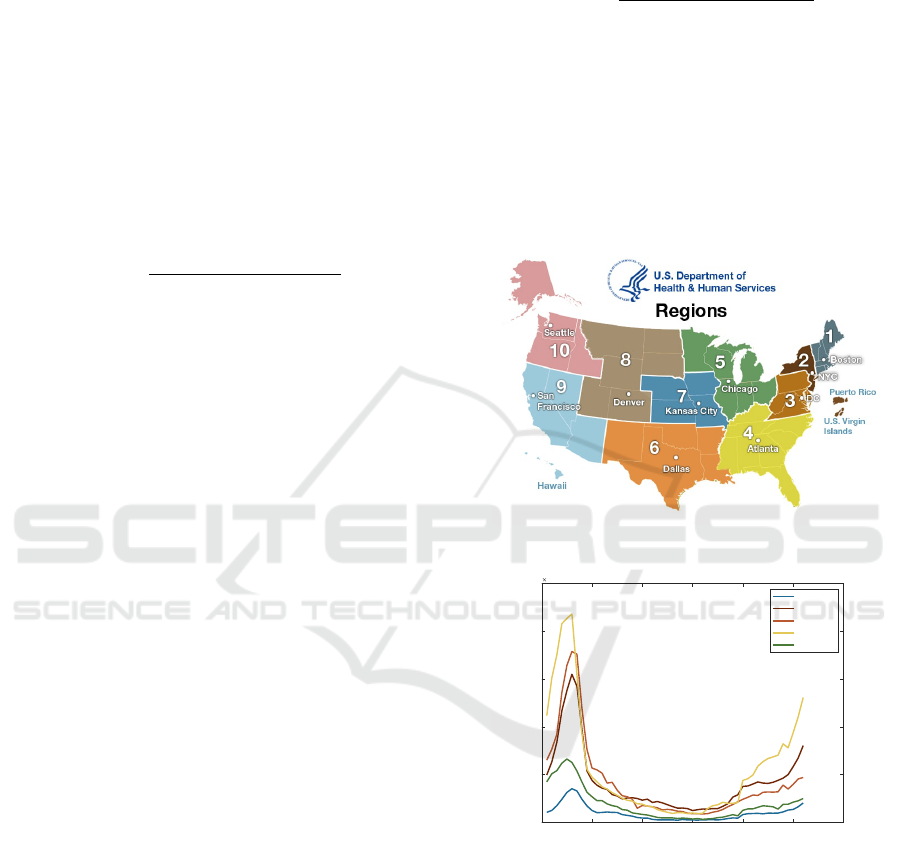
(a)

0 10 20 30 40 50 60

Week

0.5

1.5

2.5

Flu Counts

Region 1

Region 2

Region 3

Region 4

Region 5

(b)

Figure 3: Flu Counts: (a) Division Map of CDC-HHS Re-

gions Taken from HHS Website. (B) a Plot of the Trends

for ILI Counts in 2018 for Five CDC Regions.

3.2.4 Proximity Regions Factor

The geographical proximity has a strong threat of

widespread inﬂuenza outbreak. We can observe, as

shown in Fig. 3, a ﬂu trends between regions in spa-

tial proximity. We can calculate the proximity impact

on the node n by a factor coming from each neighbour

nodes which is the average of ﬂu divergence. The fac-

tor A applied at each node n, represents the average

Data-driven Model for Inﬂuenza Prediction Incorporating Environmental Effects

variation in the ﬂu counts given by the neighbour data

at time t − i. Equation. (10) is as follow:

n,i,t

j=1

i,t− j

− F

i,t− j−1

) (10)

An, i, t represents the individual adjustment for the

neighbour i to the node n at time t, is computed with

the ratio change in the previous y steps.

i,t− j

denotes the current ILI count for the neigh-

bour i at time t − j. In the study done by (Venna et al.,

2019) the y selected has to be 3, because it gave an op-

timal results. Once the individual adjustment is com-

puted, the total adjustment A

tot

n,t

at time t and node n

is the summation of weights of the individual adjust-

ment A

n,i,t

. The weights are trained using Widrow-

Hoff algorithm (Widrow and Hoff, 1988).

tot

n,t

= Σ

i=1

n,i

× A

n,i,t

(11)

N denotes the number of neighbours of data node

3.2.5 Predict Value Estimation

Final forecast value is calculated after applying the

climate variable impact from Eq. (9), the total ad-

justment factor from Eq. (11) and Eq. (6) for the air

pollution sensors to the predicted value generated by

LSTM at time t for node n as shown in Eq. (12).

f inal

n,t

= P

tot

n,t

tot

n,t

+ A

tot

n,t

+ F

LST M

n,t

(12)

4 RESULTS

In this study, we employed ARIMA a time

series-based model compared to the three pro-

posed data-driven models LSTM, proposed model:

LSTM+PS+CI+SA and ARIMA+External factors

(PS+CI+SA) on a freely available data sets about ﬂu

counts from the CDC.

We evaluate our approach on a multiple time se-

ries data: For inﬂuenza activity, we download ﬂu

counts real data sets from CDC for all ten HHS re-

gions, the data is weekly presented. We collected 52

weeks of data in ten regions from 1st week of 2018 to

the 52 nd week of 2018, the data selected for training

is from the 1st week to 46 th week. The climate data is

collected from (CDO) which is freely accessed. The

data downloaded from the CDO is weekly aggregated

for each region.

For the air pollution sensors, the data is down-

loaded from the EPA and is freely accessed, than it

was aggregated and averaged into single week.

The external predictors are weekly summarized

time series. Our samples are between 2016-2018, the

training data selected was on 80

4.1 Evaluation Criteria

To evaluate our approach for prediction performance,

we use the following evaluation metrics. Mean Ab-

solute Percentage Error (MAPE): The metric used to

measure the accuracy in percentage, is the average ab-

solute error between actual and estimated values.

MAPE =

|A − P|

|A|

(13)

Root Mean Square Percentage Error (RMSPE):

The metric used to compute the deviation between ac-

tual and predicted value and their square root.

RMSPE =

Σ(A − P)

(14)

Root Mean Square Error (RMSE): the metric used

to compute the difference between the real value and

predicted value .

RMSE =

(A − P)

× 100 (15)

N denotes the number of weeks, A denotes the ac-

tual inﬂuenza data and P denotes the predicted value.

As mentioned before, we compared the results of our

approach with the state of art ARIMA method. Also

we compared our results with the predicted value gen-

erated after application of the LSTM to prove that our

method reduces the error after LSTM.

4.2 Results for the CDC Dataset

Table. 2 shows the comparison of three models of pre-

diction: LSTM, ARIMA and our proposed approach

(LSTM + external predictors). These models are ap-

plied on all the geographical HHS regions. The table

compares the forecasting performance of the models

until 25 weeks in the future. We do three experiments

on CDC dataset for the ten regions: one for LSTM,

second for ARIMA and the third experiments for the

proposed model. We computed the performance in

terms of MAPE, RMSPE and RMSE. We can observe

an improvement of prediction accuracy after integrat-

ing the external predictors: pollution sensors, climatic

data and geographical components, to LSTM data, the

error was reduced that shows the importance of their

impact. The improvement in forecasting is noticed

from week 5 to week 15 ahead, while the ﬁrst week

IoTBDS 2020 - 5th International Conference on Internet of Things, Big Data and Security

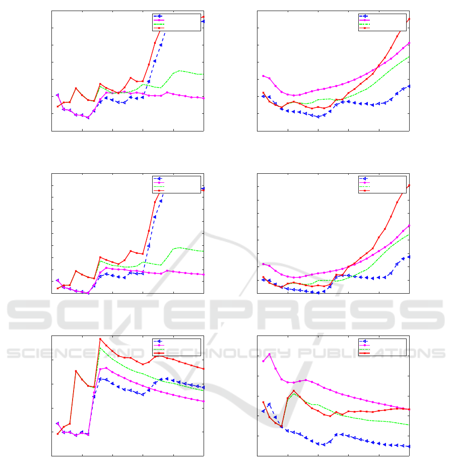
0 5 10 15 20 25

Week

MAPE

ILI Region3

Proposed Method

LSTM

ARIMA

ARIMA+External factors

(a)

0 5 10 15 20 25

Week

MAPE

ILI Region5

Proposed Method

LSTM [16]

ARIMA [7]

ARIMA+External factors

(b)

0 5 10 15 20 25

Week

RMSPE

ILI Region3

Proposed Method

LSTM

ARIMA

ARIMA+External factors

(c)

0 5 10 15 20 25

Week

100

RMSPE

ILI Region5

Proposed Method

LSTM [16]

ARIMA [7]

ARIMA+External factors

(d)

0 5 10 15 20 25

Week

500

1000

1500

2000

2500

RMSE

ILI Region3

Proposed Method

LSTM

ARIMA

ARIMA+External factors

(e)

0 5 10 15 20 25

Week

400

600

800

1000

1200

1400

1600

RMSE

ILI Region5

Proposed Method

LSTM [16]

ARIMA [7]

ARIMA+External factors

(f)

Figure 4: Comparison Using Error Metrics: MAPE (a) and (B), RMSPE (C) and (D), RMSE (E) and (F) between Region 3

(Left) and Region 5 (Right) of the Flu Prediction Models over 25 Weeks Ahead.

ahead predicted doesn’t show any signiﬁcant amelio-

ration.

Fig. 4 shows the six error charts metrics including

MAPE, RMSPE and RMSE for two regions: Region

3 and Region 5. Table. 2 is correlated with the plots

in Fig. 4 in numbers for Region 5. We can notice that

for the Region 3 for the future prediction weeks, the

MAPE error for ARIMA is less than the other mod-

els between the fourth week and the seventh week.

And our proposed model performs slightly better than

LSTM for the same region. As shown in Fig. 5, there

are ten plots, presenting the ten regions from Region

1 to Region 10 respectively, of the forecasting models

resulting from LSTM method, ARIMA and the pro-

posed compared to the actual value for the year 2018.

It can be seen that the value predicted for all the

regions of the year gives values very close to the ac-

tual one. The approach anticipates an approximate

Data-driven Model for Inﬂuenza Prediction Incorporating Environmental Effects

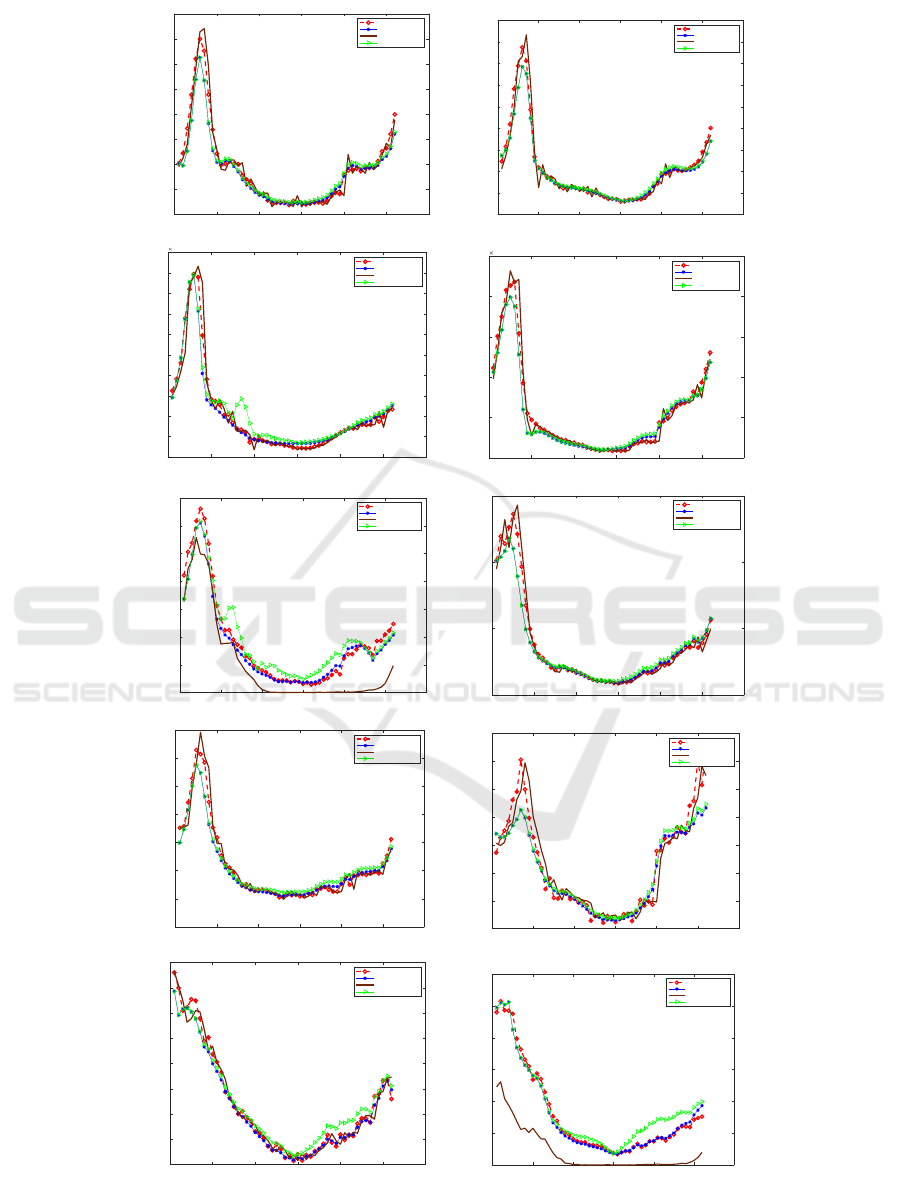
0 10 20 30 40 50 60

Week

500

1000

1500

2000

2500

3000

3500

4000

Flu Count

ILI Region1

Actual

LSTM

ARIMA

Proposed Method

0 10 20 30 40 50 60

Week

2000

4000

6000

8000

10000

12000

14000

16000

18000

Flu Count

ILI Region2

Actual

LSTM

ARIMA

Proposed Method

0 10 20 30 40 50 60

Week

0.2

0.4

0.6

0.8

1.2

1.4

1.6

1.8

Flu Count

ILI Region3

Actual

LSTM

ARIMA

Proposed Method

0 10 20 30 40 50 60

Week

0.5

1.5

2.5

Flu Count

ILI Region4

Actual

LSTM

ARIMA

Proposed Method

0 10 20 30 40 50 60

Week

1000

2000

3000

4000

5000

6000

7000

Flu Count

ILI Region5

Actual

LSTM

ARIMA

Proposed Method

0 10 20 30 40 50 60

Week

5000

10000

15000

Flu Count

ILI Region6

Actual

LSTM

ARIMA

Proposed Method

0 10 20 30 40 50 60

Week

-500

500

1000

1500

2000

2500

3000

Flu Count

ILI Region7

Actual

LSTM

ARIMA

Proposed Method

0 10 20 30 40 50 60

Week

500

1000

1500

2000

2500

3000

3500

Flu Count

ILI Region8

Actual

LSTM

ARIMA

Proposed Method

0 10 20 30 40 50 60

Week

500

1000

1500

2000

2500

3000

3500

4000

4500

Flu Count

ILI Region9

Actual

LSTM

ARIMA

Proposed Method

0 10 20 30 40 50 60

Week

500

1000

1500

2000

2500

3000

Flu Count

ILI Region10

Actual

LSTM

ARIMA

Proposed Method

Figure 5: A Plots Represent Actual and Predicted Flu Count for 10 Regions.

IoTBDS 2020 - 5th International Conference on Internet of Things, Big Data and Security

Table 2: MAPE, RMSPE and RMSE for the ILI Count Predicted Using ARIMA and Proposed Model of Region 5.

Weeks 1-week 5-week 10-week 15-week

Model MAPE RMSPE RMSE MAPE RMSPE RMSE MAPE RMSPE RMSE MAPE RMSPE RMSE

LSTM (Hochreiter and Schmidhuber, 1997) 31.95 31.95 1364 21.15 22.59 1134.9 23.92 25.02 1113.35 28.42 29.92 998.89

Proposed model 20.09 20.09 846.8 11.59 13.42 650.18 8.18 10.42 520.37 17.04 23.41 599.73

ARIMA (Choi and Thacker, 1981) 22.23 22.23 937 15.87 17.05 957.68 18.13 19.58 912.08 19.68 21.62 791.33

ARIMA+External factors 22.23 22.23 937 16.03 17.30 977.41 13.88 15.97 850.58 22.07 30.01 845.77

real-time data better than the other model. Accord-

ing to these three errors in Fig. 4 and Fig. 5, we can

say that the proposed approach is favourable for the

prediction of inﬂuenza-Like illness.

5 CONCLUSIONS

In this study, we proposed an approach to enhance in-

ﬂuenza prediction. In our contribution, ﬁrst step is the

application of LSTM as machine learning technique,

this method shows a better performance comparing

to the existing time series prediction methods. Sec-

ond step is the integration of the impacts of the exter-

nal predictors : air pollution data, climatic variables

and geographical proximity whose goal is to reduce

the error of machine learning method. We evaluated

the approach we proposed on the datasets from CDC-

HHS ILI. The proposed approach is compared with

ARIMA model. It can be seen that with the integra-

tion of external predictors in LSTM, we improved the

accuracy performance. Also, the proposed approach

may be useful for other viral illness such as Asthma,

Chickenpox and Ebola. Our future study seeks to

implement the proposed approach on Social Network

Site like Twitter and Instagram dataset.

REFERENCES

Alessa, A. and Faezipour, M. (2018). A review of in-

ﬂuenza detection and prediction through social net-

working sites. Theoretical Biology and Medical Mod-

elling, 15(1):2.

Bradley, C. A., Rolka, H., Walker, D., and Loonsk, J.

(2005). Biosense: implementation of a national

early event detection and situational awareness sys-

tem. MMWR Morb Mortal Wkly Rep, 54(Suppl):11–

19.

Choi, K. and Thacker, S. B. (1981). An evaluation

of inﬂuenza mortality surveillance, 1962–1979: I.

time series forecasts of expected pneumonia and in-

ﬂuenza deaths. American journal of epidemiology,

113(3):215–226.

Chowell, G., Miller, M., and Viboud, C. (2008). Seasonal

inﬂuenza in the united states, france, and australia:

transmission and prospects for control. Epidemiology

& Infection, 136(6):852–864.

Chowell, G., Nishiura, H., and Bettencourt, L. M. (2006).

Comparative estimation of the reproduction num-

ber for pandemic inﬂuenza from daily case notiﬁca-

tion data. Journal of the Royal Society Interface,

4(12):155–166.

Donnelly, C. F., Riley, S., Ferguson, N. M., and Anderson,

R. M. (2005). Transmission dynamics and control of

the viral aetiological agent of sars. Severe Acute Res-

piratory Syndrome: A Clinical Guide, page 111.

Dugas, A. F., Jalalpour, M., Gel, Y., Levin, S., Torcaso, F.,

Igusa, T., and Rothman, R. E. (2013). Inﬂuenza fore-

casting with google ﬂu trends. PloS one, 8(2):e56176.

Elkin, P. L., Froehling, D., Wahner-Roedler, D., Brown,

S. H., and Bailey, K. R. (2012). Comparison of nat-

ural language processing biosurveillance methods for

identifying inﬂuenza from encounter notes. Annals of

internal medicine, 156 1 Pt 1:11–8.

Gers, F. A., Schmidhuber, J., and Cummins, F. (1999).

Learning to forget: Continual prediction with lstm.

Ginsberg, J., Mohebbi, M. H., Patel, R. S., Brammer, L.,

Smolinski, M. S., and Brilliant, L. (2009). Detecting

inﬂuenza epidemics using search engine query data.

Nature, 457(7232):1012.

Hethcote, H. W. (2000). The mathematics of infectious dis-

eases. SIAM review, 42(4):599–653.

Hochreiter, S. and Schmidhuber, J. (1997). Long short-term

memory. Neural computation, 9(8):1735–1780.

Hooten, M. B., Anderson, J., and Waller, L. A. (2010). As-

sessing north american inﬂuenza dynamics with a sta-

tistical sirs model. Spatial and spatio-temporal epi-

demiology, 1(2-3):177–185.

Hu, H., Wang, H., Wang, F., Langley, D., Avram, A., and

Liu, M. (2018). Prediction of inﬂuenza-like illness

based on the improved artiﬁcial tree algorithm and ar-

tiﬁcial neural network. Scientiﬁc reports, 8(1):4895.

Keeling, M. J. and Rohani, P. (2011). Modeling infectious

diseases in humans and animals. Princeton University

Press.

Li, Q., Song, K., He, Z., Li, E., Cheng, A., and Chen, T.

(2017). The artiﬁcial tree (at) algorithm. Engineering

Applications of Artiﬁcial Intelligence, 65:99–110.

Liu, L., Han, M., Zhou, Y., and Wang, Y. (2018). Lstm

recurrent neural networks for inﬂuenza trends predic-

tion. In International Symposium on Bioinformatics

Research and Applications, pages 259–264. Springer.

Lowen, A. C., Mubareka, S., Steel, J., and Palese, P.

(2007). Inﬂuenza virus transmission is dependent on

relative humidity and temperature. PLoS pathogens,

3(10):e151.

Lowen, A. C. and Steel, J. (2014). Roles of humidity and

temperature in shaping inﬂuenza seasonality. Journal

of virology, 88(14):7692–7695.

Data-driven Model for Inﬂuenza Prediction Incorporating Environmental Effects

Lu, Y., Garcia, R., Hansen, B., Gleicher, M., and Maciejew-

ski, R. (2017). The state-of-the-art in predictive visual

analytics. In Computer Graphics Forum, volume 36,

pages 539–562. Wiley Online Library.

Luo, W. (2016). Visual analytics of geo-social interaction

patterns for epidemic control. International journal of

health geographics, 15(1):28.

Nishiura, H. (2011). Real-time forecasting of an epidemic

using a discrete time stochastic model: a case study

of pandemic inﬂuenza (h1n1-2009). Biomedical engi-

neering online, 10(1):15.

Paul, M. J., Sarker, A., Brownstein, J. S., Nikfarjam, A.,

Scotch, M., Smith, K. L., and Gonzalez, G. (2016).

Social media mining for public health monitoring and

surveillance. In Biocomputing 2016: Proceedings of

the Paciﬁc symposium, pages 468–479. World Scien-

tiﬁc.

Ram, S., Zhang, W., Williams, M., and Pengetnze, Y.

(2015). Predicting asthma-related emergency depart-

ment visits using big data. IEEE journal of biomedical

and health informatics, 19(4):1216–1223.

Santillana, M., Nguyen, A. T., Dredze, M., Paul, M. J.,

Nsoesie, E. O., and Brownstein, J. S. (2015). Combin-

ing search, social media, and traditional data sources

to improve inﬂuenza surveillance. PLoS computa-

tional biology, 11(10):e1004513.

Shaman, J., Karspeck, A., Yang, W., Tamerius, J., and Lip-

sitch, M. (2013). Real-time inﬂuenza forecasts dur-

ing the 2012–2013 season. Nature communications,

4:2837.

Siegelmann, H. T. and Sontag, E. D. (1991). Turing com-

putability with neural nets.

Signorini, A., Segre, A. M., and Polgreen, P. M. (2011).

The use of twitter to track levels of disease activity

and public concern in the u.s. during the inﬂuenza a

h1n1 pandemic. PLOS ONE, 6:1–10.

Soebiyanto, R. P., Adimi, F., and Kiang, R. K. (2010).

Modeling and predicting seasonal inﬂuenza transmis-

sion in warm regions using climatological parameters.

PloS one, 5(3):e9450.

Tsui, F., Wagner, M., Cooper, G., Que, J., Harkema, H.,

Dowling, J., Sriburadej, T., Li, Q., Espino, J. U., and

Voorhees, R. (2011). Probabilistic case detection for

disease surveillance using data in electronic medical

records. Online journal of public health informatics,

3(3).

Venna, S. R., Tavanaei, A., Gottumukkala, R. N., Raghavan,

V. V., Maida, A. S., and Nichols, S. (2019). A novel

data-driven model for real-time inﬂuenza forecasting.

IEEE Access, 7:7691–7701.

Wagner, M. M., Moore, A. W., and Aryel, R. M. (2011).

Handbook of biosurveillance. Elsevier.

Widrow, B. and Hoff, M. E. (1988). Adaptive switching

circuits.

IoTBDS 2020 - 5th International Conference on Internet of Things, Big Data and Security