Meta-parameters Exploration
for Unsupervised Event-based Motion Analysis
Ve
¨
ıs Oudjail
1
and Jean Martinet
2 a
1
Univ. Lille, CNRS, Centrale Lille, UMR 9189 – CRIStAL, F-59000, Lille, France
2
Universit
´
e C
ˆ
ote d’Azur, CNRS, I3S, France
Keywords:
Motion Analysis, Spiking Neural Networks, Event-based Sensor, Parameter Exploration.
Abstract:
Being able to estimate motion features is an essential step in dynamic scene analysis. Optical flow typically
quantifies the apparent motion of objects. Motion features can benefit from bio-inspired models of mammalian
retina, where ganglion cells show preferences to global patterns of direction, especially in the four cardinal
translatory directions. We study the meta-parameters of a bio-inspired motion estimation model using event
cameras, that are bio-inspired vision sensors that naturally capture the dynamics of a scene. The motion
estimation model is made of an elementary Spiking Neural Network, that learns the motion dynamics in a non-
supervised way through the Spike-Timing-Dependent Plasticity. After short simulation times, the model can
successfully estimate directions without supervision. Some of the advantages of such networks are the non-
supervised and continuous learning capabilities, and also their implementability on very low-power hardware.
The model is tuned using a synthetic dataset generated for parameter estimation, made of various patterns
moving in several directions. The parameter exploration shows that attention should be given to model tuning,
and yet the model is generally stable over meta-parameter changes.
1 INTRODUCTION
Motion features are useful in a wide range of com-
puter vision tasks, and traditionally requires the ex-
traction and processing of keyframes, to define mo-
tion descriptors such as optical flow. Determining the
optical flow consists in estimating the elementary dis-
placements of interest points in a video stream.
High precision approaches are based on deep
learning (Ilg et al., 2017). However, most solu-
tions use a large amount of annotated data as part of
their supervised learning. Besides, training deep net-
works use significant computing resources that cause
a significant energy cost. Spiking Neural Networks
(SNN), however, allow unsupervised learning: the
Spike-Timing-Dependent Plasticity (STDP) learning
rule used in SNN training is not supervised. Un-
like the stochastic gradient descent used in conven-
tional networks, which is a global rule, STDP is lo-
cal. This locality makes it possible to design low-
power massively parallel hardware circuits. However,
the challenge is to be able to use this model in vi-
sion tasks with performances that rival state-of-the-art
a
https://orcid.org/0000-0001-8821-5556
methods. One of the difficulties is the configuration
of the model; indeed, the adjustment is very sensitive
and has a direct impact on system performance. A
fine-tuning phase must be carried out to find the right
setting, which makes it difficult to use SNN.
In this paper, we investigate temporal data analy-
sis with SNN for video. We consider the event cam-
eras such as Dynamic Vision Sensors (DVS) (Licht-
steiner et al., 2008). These sensors output an Ad-
dress Event Representation (AER), each pixel indi-
vidually encodes positive and negative intensity vari-
ations – every change triggers an event that is trans-
mitted asynchronously. There are two types of events:
ON-events for positive variations and OFF-events for
negative variations. Such a representation is well
adapted to SNN, because the events resemble spikes,
and therefore they can be used to feed the network in
a straightforward manner. Our objective is to study
elementary network structures able to classify a mo-
tion stimulus inside a small window. We success-
fully trained simple one-layer fully-connected feed-
forward spiking neural networks to recognise the mo-
tion orientation of binary patterns in a 5 × 5 window,
in an unsupervised manner.
Oudjail, V. and Martinet, J.
Meta-parameters Exploration for Unsupervised Event-based Motion Analysis.
DOI: 10.5220/0009324908530860
In Proceedings of the 15th International Joint Conference on Computer Vision, Imaging and Computer Graphics Theory and Applications (VISIGRAPP 2020) - Volume 4: VISAPP, pages
853-860
ISBN: 978-989-758-402-2; ISSN: 2184-4321
Copyright
c
 2022 by SCITEPRESS – Science and Technology Publications, Lda. All rights reserved
853

We considered several patterns, with a varying
number of input spiking pixels. We explored the
meta-parameter space in order to exhibit successful
settings. Through this exploration, we identified key
meta-parameters that have the most impact. We show
that the neuron activation threshold is the most influ-
encing meta-parameter for the performance. We also
show the need to adjust the threshold value when the
number of active input pixels changes.
The remainder of the paper is organised as fol-
lows: Section 2 discusses the use of SNN in vision,
namely for image and video classification, Section 3
describes the core model, by giving details regarding
the dataset, the network structure, and the experimen-
tal protocol, Section 4 shows and discusses the meta-
parameter exploration, and Section 5 concludes the
paper and discusses future work.
2 RELATED WORK
2.1 Spiking Neural Networks
Spiking Neural Networks represent a special class of
artificial neural networks (Maass, 1997), where neu-
rons communicate by sequences of spikes (Ponulak
and Kasinski, 2011). SNN have long been used in the
neuroscience community as a reliable model to pre-
cisely simulate biology and understand brain mecha-
nisms (Paugam-Moisy and Bohte, 2012).
Contrary to widely-used deep convolutional neu-
ral networks, spiking neurons do not fire at each prop-
agation cycle, but rather fire only when their activa-
tion level (or membrane potential, an intrinsic qual-
ity of the neuron related to its membrane electri-
cal charge) reaches a specific threshold value. SNN
do not rely on stochastic gradient descent and back-
propagation. Instead, neurons are connected through
synapses, that implement a learning mechanism in-
spired from biology. The STDP is a rule that up-
dates synaptic weights according to the spike timings,
and increases the weight when a presynaptic spike oc-
curs just before a postsynaptic spike (within a few
milliseconds). Therefore, the learning process is in-
trinsically not supervised, and SNN can be success-
fully used to detect patterns in data in an unsupervised
manner (Oudjail and Martinet, 2019; Bichler et al.,
2012; Hopkins et al., 2018).
Several studies have attempted to reproduce and
apply to SNN several mechanisms that contribute to
the success of deep networks, such as the stochastic
gradient descent (Lee et al., 2016) or deep convolu-
tional architectures (Cao et al., 2015; Tavanaei and
Maida, 2017). However, such approaches do
not benefit from the unsupervised advantage of
STDP.
2.2 Event Video Classification
In addition, SNN are increasingly used in data
processing because of their implementability on
low-energy hardware such as neuromorphic circuits
(Merolla et al., 2014; Sourikopoulos et al., 2017;
Kreiser et al., 2017). SNN have been used in
vision-related tasks (Masquelier and Thorpe, 2007),
and some researchers have addressed standard vision
datasets with SNN and DVS by converting them into
an event representation, such as Poker-DVS, MNIST-
DVS (Serrano-Gotarredona and Linares-Barranco,
2015), N-MNIST (Orchard et al., 2015), and CIFAR-
DVS (Li et al., 2017).
More specifically in motion analysis, several at-
tempts to apply SNN for video classification or for
more specific video-related tasks exist. Bichler et al.
(Bichler et al., 2012) have used a feed-forward SNN
capable of recognising the movement of a ball among
8 discretised directions from event data. They also
show in another experiment that SNN can be used to
count cars passing on a highway lane. The data is
captured with a DVS.
Orchard et al. (Orchard et al., 2013) developed a
system to extract the optical flow from an event video
sequence. A simple test setup was constructed con-
sisting of a black pipe spinning in front of a white
background. This setup is used for testing different
motion speeds and directions. In their approach, they
use 5 × 5 receptive fields, with neurons that are sen-
sitive to certain motion directions and speeds (8 di-
rections and 8 speeds), with the assumption that the
speed is fixed and constant. In the model, they in-
tegrate, synaptic delays in order to be sensitive to
spatio-temporal patterns. All parameters are fixed at
the beginning, so there is no learning in their model.
Zhao et al. (Zhao et al., 2015) combine an HMAX
and SNN feed-forward architecture to recognise the
following 3 human actions from event videos: bend-
ing, walking and standing/sitting, where the types of
movement can be simplified by diagonal, horizontal
and vertical motions.
Amir et al. (Amir et al., 2017) have designed a
demo for recognising more than 10 hand gestures in
real time with a low-energy consumption, by exploit-
ing a neuromorphic processor with a capacity of one
million neurons, running an SNN coupled to a pre-
trained CNN. Such a system reached a 96.5% success
rate.
VISAPP 2020 - 15th International Conference on Computer Vision Theory and Applications
854

2.3 Relation to Our Work
All previously mentioned work use both ON- and
OFF-event types. With this rich information, if we
assume a constant intensity for objects and back-
grounds, the object motion can be inferred in short
temporal windows. Let us take the example of a white
ball moving towards the right before a darker back-
ground. The right edge of the ball will generate a set
of ON-events and the opposite edge (left) will simul-
taneously generate a set of OFF events. In this setting,
the motion recognition problem boils down to a static
pattern recognition problem, because the very motion
is encoded in a static way. Moreover, if the object
is either large or close to the sensor, then ON-events
and OFF-events will be much separated in space, or
even separated in time (i.e. they will not occur si-
multaneously in the sensor) if the object is larger than
the sensor’s field of view, making it almost impossi-
ble for such static approaches to infer a motion. In
this paper, we study focus on learning dynamic ob-
ject motions. Therefore, we deliberately ignore the
event types, and we use a single event type, indicat-
ing either types of intensity variation. The purpose is
to train detectors that are sensitive to certain stimuli
sequences. To achieve this, we design and use ele-
mentary network structures whose output layer is ca-
pable of learning the direction of a given input binary
texture in motion.
3 METHODOLOGY
We wish to investigate the impact of parameters tun-
ing of a simple feed-forward network on the ability to
learn the motion direction of a binary texture pattern.
This section relates how the data was generated, gives
details of the network structure and default parame-
ters, and describes the experimental protocol.
3.1 Synthetic Event Data
Standard Address Event Representation (AER) en-
codes positive and negative pixel-wise luminosity
variation in the form of ON- and OFF-events. In our
model, we used a simplified representation merging
both types into a single type of event. We generated
synthetic event data mimicking the displacement of
simple texture patterns in four directions (NORTH,
SOUTH, WEST, EAST) inside a 5 × 5 window. Fig-
ure 1 shows an illustration of a square pattern motion
in the EAST direction.
Therefore, we have four classes for each pattern.
The speed is set to 480 pixels/s as in the experiments
Figure 1: Illustration of a pattern motion in the EAST di-
rection.
described in (Bichler et al., 2012), and one sample
input corresponds to a 30-ms duration of stimulation.
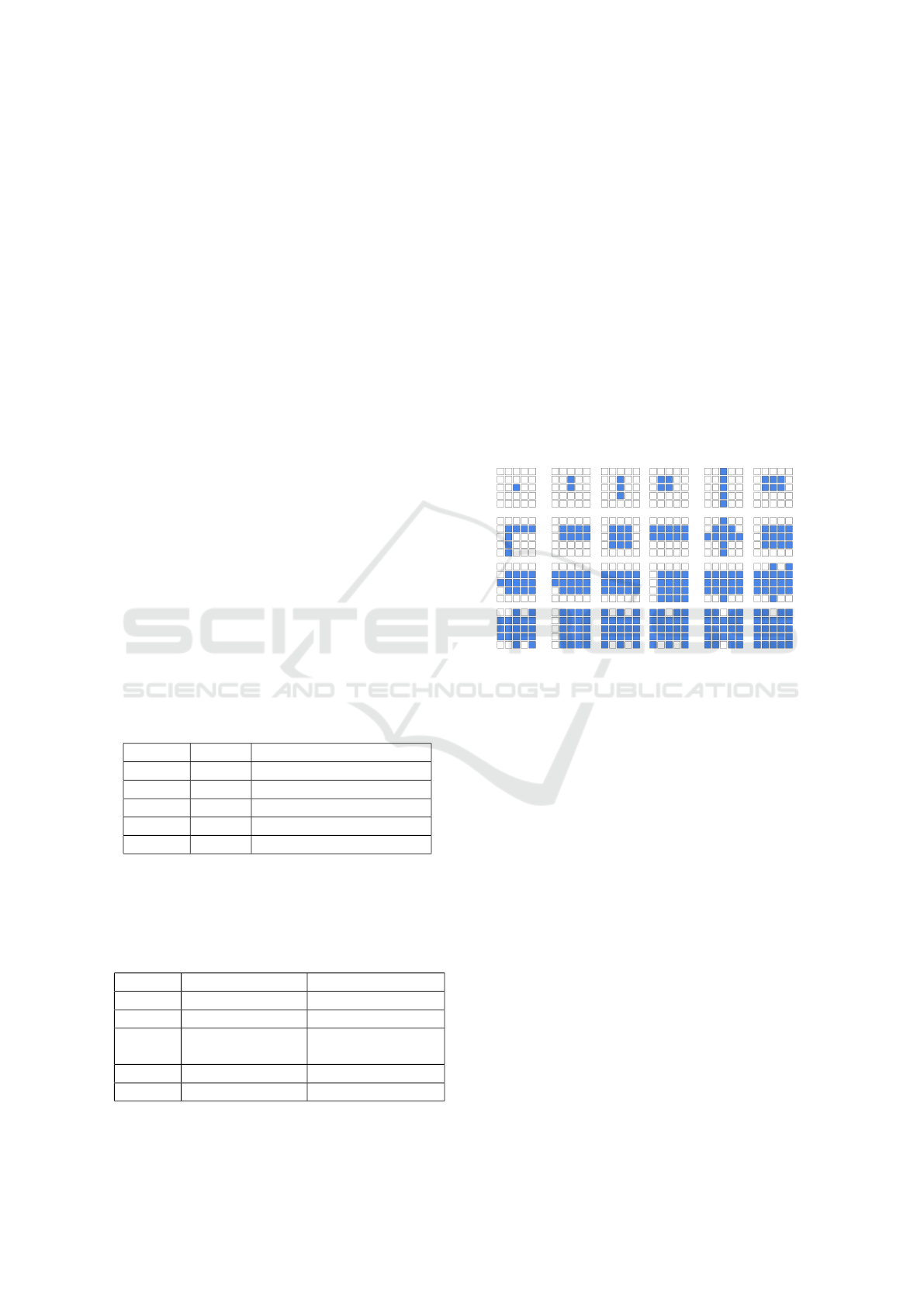
We consider several patterns with varying number
of input spiking pixels, ranging from 1 to 24, as shown
Figure 3.
3.2 Network Details
Our network is a simple one-layer fully-connected
feed-forward SNN, that takes the event data as a 5× 5
continuous input (as illustrated Figure 2), and whose
output layer is a vector encoding motion classes.
Figure 2: Topological overview of the network.
Among several neuron models, we use the Leaky-
Integrate-and-Fire (LIF) model – see (Ponulak and
Kasinski, 2011). This model integrates input spikes
to its membrane potential V . When V exceeds a pre-
defined threshold V
thres
, then an output spike is trig-
gered and V is reset to 0. Otherwise, V decays with
time (unless other input spikes occur), at a certain rate
τ
leak
. The model is defined as follows:
τ
leak
∂V
∂t
= −V +
∑
i∈S
V
i
δ(t − t
i
)
V ← 0 when V ≥ V
thres
(1)
S is the set of incoming spikes, V
i
the voltage of the i
th
spike, t
i
the timestamp of the i
th
spike and δ the Dirac
function.
In this model, the synapses modulate the spikes
voltage V
i
that passes through connections according
to a synapse weight w. The learning rule, common
to all the simulations presented in this paper, is a sim-
plified Spike-timing-dependent plasticity (STDP) rule
(Bichler et al., 2012).
∆t = t
post
− t
pre
∆w = ST DP(∆t) =

∆w
+
if 0 ≤ ∆t ≤ T
LTP
∆w
−
otherwise
(2)
Meta-parameters Exploration for Unsupervised Event-based Motion Analysis
855

where t
pre
(resp. t
post
) represents the presynaptic
(resp. postsynaptic) spike timestamp, and T
LTP
is
the width of the potentiation window (LTP stands for
Long Term Potentiation). If the postsynaptic spike oc-
curs within T
LTP
ms after the presynaptic spike, the
synapse is potentiated by ∆w
+
mV. Otherwise, other
values of ∆t trigger a Long Term Depression (LTD),
where the synapse is depressed by ∆w
−
mV.
In our experiments, parameters are set individu-
ally for each synapse in the following way: a min-
imum and a maximum bound are set randomly, and
the initial value of the synapse is chosen randomly in-
side the bounds. Moreover, ∆w
−
and ∆w
+
are also set
randomly for each synapse, with the only constraint
that ∆w
−
< ∆w
+
. Moreover, our model includes 3
bio-inspired mechanisms:
• a competition constraint that prevents all out-
put units to learn the same pattern: neurons are
equipped with lateral inhibition capability, where
an active neuron prevents its neighbours to spike
during a given time T
inhibit
;
• refractory periods to prevent a single output unit
to continuously burst without giving other units a
chance to emit output spikes;
• synaptic delays to avoid that all incoming spikes
occur simultaneously.
We implemented this network using Brian2 SNN sim-
ulator (Goodman and Brette, 2009) with parameters
similar to (Bichler et al., 2012).
Table 1: Value of the default neuronal parameters.
Param. Value Description
V
thres
20 mV Action potential threshold
T
LTP
2 ms Long Term Potentiation
T
re f rac
10 ms Refractory period
T
inhibit
20 ms Inhibition time
τ
leak
5 Leak rate
Table 2: Mean (µ) and standard deviation (σ) for the synap-
tic parameters, for all the simulations in this paper. The
parameters are randomly chosen for each synapse at the be-
ginning of the simulations, using the normal distribution.
Note that the weights are expressed in mV, because it is
synapses that deliver tension.
Param. µ σ Description
w
min
0.02 mV 0.002 Minimum weight
w
max
6.00 mV 2 Maximal weight
w 50% 30% Weight (normal-
ized with limits)
∆w
+
10% 5% LTP
∆w
−
5% 2.5% LTD
3.3 Protocol
We demonstrate the capabilities for model with sev-
eral types of input patterns. We show that the model
is be able to differentiate between NORTH, SOUTH,
WEST, EAST directions for the considered patterns
(four distinguishable classes).
During a simulation, we alternate learning phases,
corresponding to the period when the network evolves
by modifying its weights according to stimuli, and test
phases in which the STDP is disabled. It is during the
test phases that measurements are made.
We explore the 2 following network parameters :
neuron activation threshold and neuron leak. Also,
we assess the impact of the number of input spiking
pixels (N) by using 24 patterns (see Figure 3) where
N ranges from 1 to 24.
Figure 3: Twenty-four input patterns used in our experi-
ments.
3.4 Score Assessment
For each simulation, output codes are generated in
the following way : an output neuron is assigned 1
if and only if at least one spike is triggered during
the test phase. All classes are presented sequentially
to the network and we observe the output codes, as
illustrated Figure 4. With these output codes, a score
can be estimated by comparing the different codes and
identifying those that are distinguishable. Indeed, we
are interested in distinguishing between input classes.
Therefore, the score value is between 0 and 4.
Note that the output code with only zeros does not
represent a class. A score value is obtained during
each test phase. Given the random weights initialisa-
tion, we run 10 executions per configuration in order
to obtain a reliable estimation of the score. There are
40 test phases per run ; for each test phase, the scores
of all runs are averaged.
VISAPP 2020 - 15th International Conference on Computer Vision Theory and Applications
856

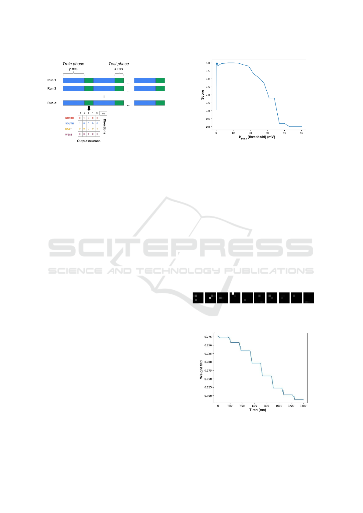
Figure 4: Training phases have a duration of y ms, they cor-
respond to the presentation of one class. Test phases have
a duration of x ms, they correspond to the presentation of a
sequence of all four classes.
4 EXPERIMENTAL RESULT
The aim of the unsupervised training step is to ad-
just synaptic weights so as to reach a network state
where the outputs precisely distinguish between input
classes. This means that some output layer neurons
would become specialised in detecting a particular in-
put class. A necessary situation of specialisation is
when some synaptic weights have converged to val-
ues close to 0 or 1, indicating that the corresponding
output neuron has become either insensitive or sen-
sitive to the corresponding input spiking pixel, there-
fore proving a specialisation of the network toward a
particular stimulus.
During simulations, we observe the output activity
of the network as well as all the synaptic weight val-
ues. In particular, we monitor both output codes for
classes during test phases and the synaptic weights
evolution (more precisely: the standard deviation of
synaptic weights). The aim is to measure the impact
of the different parameters of the model during train-
ing. During the different experiments, the parameters
that do not vary have a value indicated in the Table 1.
4.1 Impact of the Threshold V
thres
In order to assess the impact of threshold (V
thres
), we
show the score value when varying V
thres
∈ [0, 50] mV
(Figure 5).
We see that when the threshold has a zero value
i.e. all output neurons will emit a spike when re-
ceiving a presynaptic spike, regardless of the value
of their (strictly positive) synaptic weights. In this
case, the neurons are sensitive to all input stimuli and
cannot distinguish between classes, hence the score
is 1 (remember that the score denotes the number of
classed that can be distinguished). Since the output
Figure 5: Evolution of the score when varying V
thres
.
spikes have no correlation with the incoming spikes,
following the STDP learning rule, this configuration
results in a succession of LTD decreasing the synap-
tic connections to such an extent that most values are
close to w
min
. An example of such a situation of low
synaptic connection values for a network containing
10 output neurons is displayed Figure 6, where each
matrix represents the normalised synaptic weights be-
tween one of the 10 output neurons and the 25 input
neurons. This representation preserves the spatial ar-
rangement of the input neurons. Light/dark zones in-
dicate weights of sensitive/insensitive connections of
output neurons. We can observe that most synaptic
weights have become 0, indicating mainly insensitive
output neurons. We also display Figure 7 the evo-
lution curve of the standard deviations of the synaptic
weights during the simulation. This curve shows a de-
creasing standard deviation, which further confirms a
wrong parameter setting.
Figure 6: Illustration of synaptic weights for the network
when V
thres
= 0mV (non ideal case).
Figure 7: Evolution of the global standard deviation of
synaptic weights during a simulation (non ideal case). The
plateaus correspond to the different test phases, where the
STDP learning rule is disabled.
Meta-parameters Exploration for Unsupervised Event-based Motion Analysis
857

For the following values, in particular, for those
between 0.1 and 0.9 mV reach the score of 4.
For thresholds with high values, the neuron’s
membrane potential has difficulty reaching this volt-
age or even more, even in the most favourable con-
figurations (high synaptic weights), which leads to a
decrease or even absence of output activity from the
network.
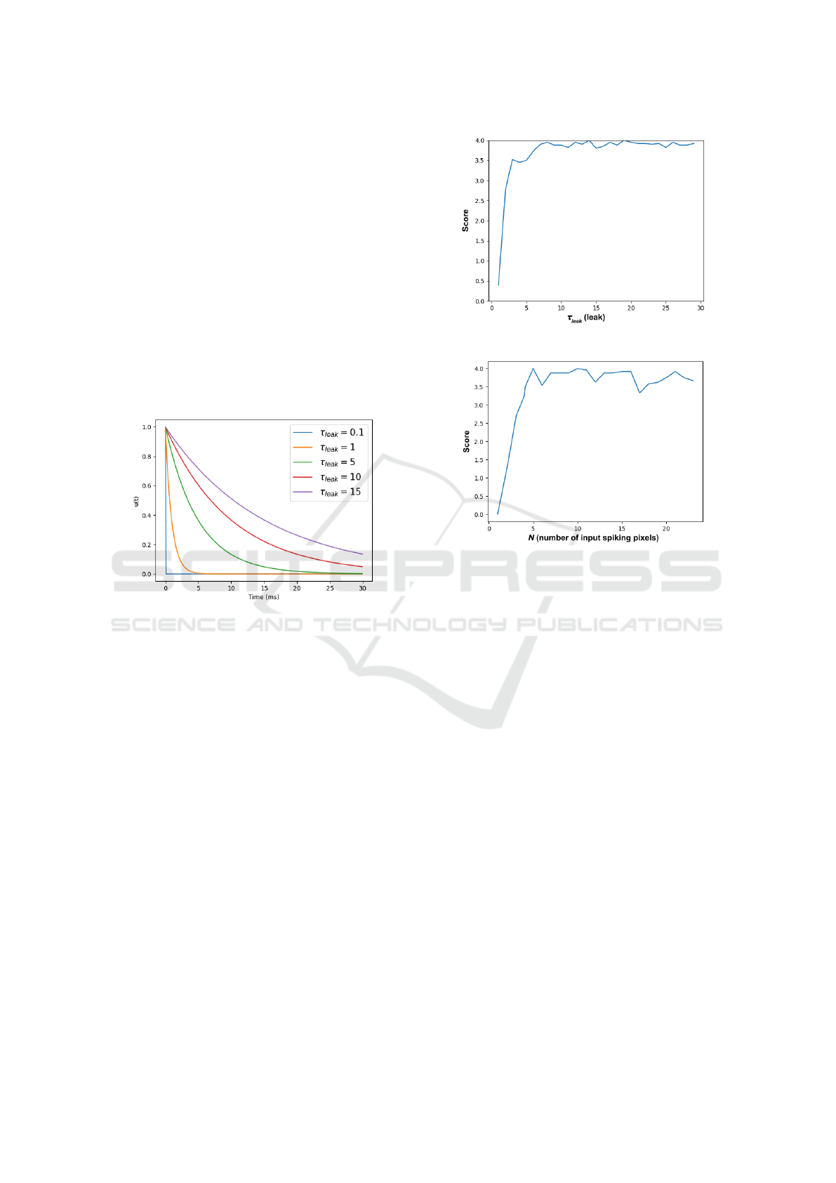
4.2 Impact of the Leak τ
leak
The leak can be pictured as a water leak from a
pierced bottle. It makes the membrane potential de-
crease with time, until a rest value is reached. With
the water analogy, τ
leak
is a coefficient that would be
inversely proportional to the size of the hole in the
leaky bottle – see Figure 8.
Figure 8: Leak with different values of τ
leak
.
In order to assess the impact of neurons’ leak,
we show in Figure 9 the score values when varying
τ
leak
∈ [0, 30]. When τ
leak
is small (resp. large) it
means that the leak is fast (resp. slow). When the
leak value is low, it causes the obtained score to be
also low because the decrease in membrane potential
is fast and it prevents the output neurons’ membrane
to reach the activation threshold. When the leak value
is larger, especially when it reaches a certain value (9,
in our case), the parameter no longer influences the
score, that stabilises around the optimal score value
of 4. In such case, a LIF neuron with a large leak is
an approximation of IF neuron (i.e. a neuron with no
leak).
4.3 Impact of the Number of Input
Spiking Pixels N
In order to assess the impact of the number of input
spiking pixels (N), we use the patterns shown Fig-
ure 3, where the number of input spiking pixels varies
from 1 to 24. Figure 10 shows the corresponding
score values.
Figure 9: Evolution of the score when varying τ
leak
.
Figure 10: Evolution of the score when varying the number
of input spiking pixels N.
The number of input spiking pixels (N) has an in-
fluence on the score, particularly in situations where
the number of pixels is in [1, 3], a score is obtained
between [0, 3]. In this case of low N values, the input
does not produce enough spikes to activate the output
neurons.
4.4 Joint Impact of the Threshold V
thres
and Leak τ
leak
In order to assess the joint impact of threshold (V
thres
)
and neuron’s leak (τ
leak
), we show in Figure 11 the
score value when varying V
thres
∈ [1mV, 35mV ] and
τ
leak
∈ [0, 15].
The same observation can be made as when τ
leak
is low. However, this can be offset by adjusting the
threshold to lower values. To support this point, by
choosing a threshold V
thres
∈ [20mV, 35mV ], we ob-
serve that by increasing the leak coefficient, the scores
improve.
This behaviour comes from the fact that both pa-
rameters influence the decision of a neuron to emit a
spike or not. The leak controls an aspect of the evo-
lution of the membrane potential and the threshold
controls the value that the membrane potential volt-
age must reach for there to be a spike at the output.
VISAPP 2020 - 15th International Conference on Computer Vision Theory and Applications
858

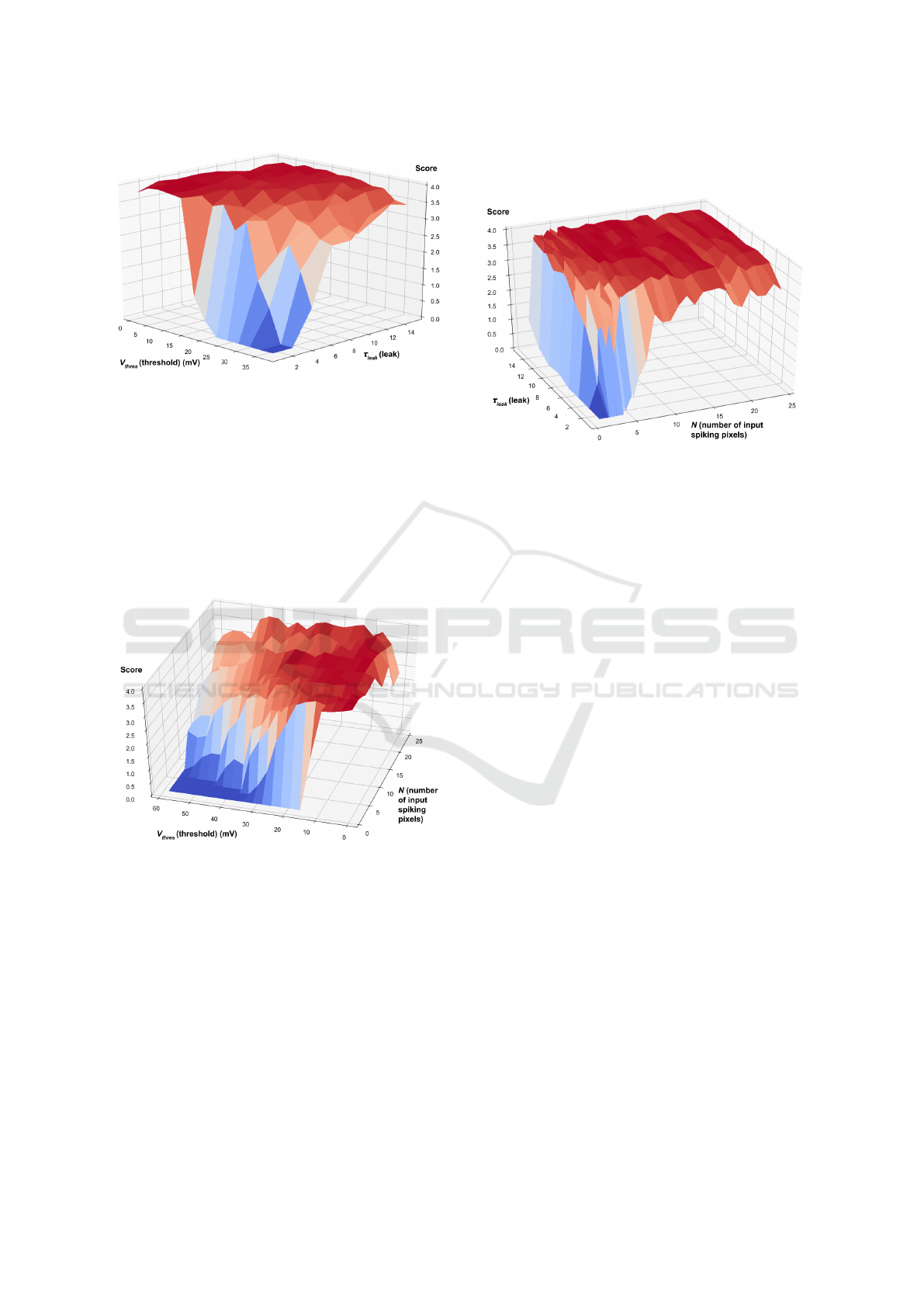
Figure 11: Evolution of the score when varying the thresh-
old V
thres
and leak τ
leak
.
4.5 Joint Impact of the Number of
Input Spiking Pixels N and
Threshold V
thres
In order to jointly assess the impact of the number of
input spiking pixels (N) and the threshold (V
thres
), we
show the score value when varying N ∈ [1, 24] and
V
thres
∈ [1mV, 50mV ] (Figure 12).
Figure 12: Evolution of the score when varying the number
of input spiking pixels N and threshold V
thres
.
When observing the output graph, we see that
the parameters configurations yielding low scores are
those where V
thres
is high and N is small. Indeed, pat-
terns with a number of pixels less than 4 are very sen-
sitive to threshold setting. The best threshold on aver-
age is a low threshold at 10 mV.
4.6 Joint Impact of the Number of Input
Spiking Pixels N and Leak τ
leak
In order to jointly assess the impact of the number
of input spiking pixels (N) and the leak (τ
leak
), we
show the score value when varying N ∈ [1, 24] and
τ
leak
∈ [1, 15] (Figure 13).
Figure 13: Evolution of the score when varying the number
of input spiking pixels N and leak τ
leak
.
There is a clear influence of both N and τ
leak
on the
output score, even though the impact is less important
than the threshold V
thres
. Most score values are close
to 4, except when τ
leak
< 4 or N < 2. We notice that
when both τ
leak
and N are small (i.e. fast leak and
little input activity), the score becomes null.
5 CONCLUSION
In this paper, we have presented a study or meta-
parameters impact for an approach of unsupervised
motion analysis. Our contributions include the design
and training of a Spiking Neural Network to classify
event video data, with a parameter exploration regard-
ing the threshold V
thres
, the leak leak τ
leak
, and the
number of input spiking pixels N. The aims is to es-
timate the impact of the parameters N, V
thres
and τ
leak
on the model for the motion classification task.
In future work, we wish to explore two orthogonal
directions:
• target invariance regarding motion speed, possibly
by further exploiting synaptic delays so that sev-
eral speeds will trigger the same network output,
• target speed sensitivity, with a dedicated architec-
ture whose output units are specialised for distinct
speed classes.
We will refine the method of evaluating the efficiency
of the network, using a classifier on the output spikes.
Also, we will evaluate our model on real-world event
data.
In a longer term, we wish to use such elemen-
tary networks as local motion detectors, to be laid out
Meta-parameters Exploration for Unsupervised Event-based Motion Analysis
859

in layers or other topologies to enable unsupervised
analysis of more complex motion patterns.
ACKNOWLEDGEMENTS
This work has been partly funded by IRCICA (Univ.
Lille, CNRS, USR 3380 IRCICA, Lille, France).
REFERENCES
Amir, A., Taba, B., Berg, D. J., Melano, T., McKinstry,
J. L., Di Nolfo, C., Nayak, T. K., Andreopoulos, A.,
Garreau, G., Mendoza, M., et al. (2017). A low
power, fully event-based gesture recognition system.
In CVPR, pages 7388–7397.
Bichler, O., Querlioz, D., Thorpe, S. J., Bourgoin, J.-P.,
and Gamrat, C. (2012). Extraction of temporally
correlated features from dynamic vision sensors with
spike-timing-dependent plasticity. Neural Networks,
32:339–348.
Cao, Y., Chen, Y., and Khosla, D. (2015). Spiking deep
convolutional neural networks for energy-efficient ob-
ject recognition. International Journal of Computer
Vision, 113(1):54–66.
Goodman, D. F. and Brette, R. (2009). The brian simulator.
Frontiers in neuroscience, 3:26.
Hopkins, M., Pineda-Garc
´
ıa, G., Bogdan, P. A., and Furber,
S. B. (2018). Spiking neural networks for computer
vision. Interface Focus, 8(4):20180007.
Ilg, E., Mayer, N., Saikia, T., Keuper, M., Dosovitskiy, A.,
and Brox, T. (2017). Flownet 2.0: Evolution of optical
flow estimation with deep networks. In CVPR 2017,
pages 1647–1655. IEEE.
Kreiser, R., Moraitis, T., Sandamirskaya, Y., and Indiveri,
G. (2017). On-chip unsupervised learning in winner-
take-all networks of spiking neurons. In Biomedi-
cal Circuits and Systems Conference (BioCAS), 2017
IEEE, pages 1–4. IEEE.
Lee, J. H., Delbruck, T., and Pfeiffer, M. (2016). Training
deep spiking neural networks using backpropagation.
Frontiers in neuroscience, 10:508.
Li, H., Liu, H., Ji, X., Li, G., and Shi, L. (2017). Cifar10-
dvs: an event-stream dataset for object classification.
Frontiers in neuroscience, 11:309.
Lichtsteiner, P., Posch, C., and Delbruck, T. (2008). A
128×128 120 db 15µ s latency asynchronous tempo-
ral contrast vision sensor. IEEE journal of solid-state
circuits, 43(2):566–576.
Maass, W. (1997). Networks of spiking neurons: the third
generation of neural network models. Neural net-
works, 10(9):1659–1671.
Masquelier, T. and Thorpe, S. J. (2007). Unsupervised
learning of visual features through spike timing de-
pendent plasticity. PLoS computational biology,
3(2):e31.
Merolla, P. A., Arthur, J. V., Alvarez-Icaza, R., Cassidy,
A. S., Sawada, J., Akopyan, F., Jackson, B. L., Imam,
N., Guo, C., Nakamura, Y., et al. (2014). A mil-
lion spiking-neuron integrated circuit with a scal-
able communication network and interface. Science,
345(6197):668–673.
Orchard, G., Benosman, R., Etienne-Cummings, R., and
Thakor, N. V. (2013). A spiking neural network ar-
chitecture for visual motion estimation. In Biomedi-
cal Circuits and Systems Conference (BioCAS), 2013
IEEE, pages 298–301. IEEE.
Orchard, G., Jayawant, A., Cohen, G. K., and Thakor, N.
(2015). Converting static image datasets to spiking
neuromorphic datasets using saccades. Frontiers in
neuroscience, 9:437.
Oudjail, V. and Martinet, J. (2019). Bio-inspired event-
based motion analysis with spiking neural networks.
In VISAPP 2019, pages 389–394.
Paugam-Moisy, H. and Bohte, S. (2012). Computing with
spiking neuron networks. In Handbook of natural
computing, pages 335–376. Springer.
Ponulak, F. and Kasinski, A. (2011). Introduction to spik-
ing neural networks: Information processing, learning
and applications. Acta neurobiologiae experimentalis,
71(4):409–433.
Serrano-Gotarredona, T. and Linares-Barranco, B. (2015).
Poker-dvs and mnist-dvs. their history, how they were
made, and other details. Frontiers in neuroscience,
9:481.
Sourikopoulos, I., Hedayat, S., Loyez, C., Danneville, F.,
Hoel, V., Mercier, E., and Cappy, A. (2017). A 4-
fj/spike artificial neuron in 65 nm cmos technology.
Frontiers in neuroscience, 11:123.
Tavanaei, A. and Maida, A. S. (2017). Multi-layer unsuper-
vised learning in a spiking convolutional neural net-
work. In IJCNN 2017, pages 2023–2030. IEEE.
Zhao, B., Ding, R., Chen, S., Linares-Barranco, B., and
Tang, H. (2015). Feedforward categorization on aer
motion events using cortex-like features in a spiking
neural network. IEEE Trans. Neural Netw. Learning
Syst., 26(9):1963–1978.
VISAPP 2020 - 15th International Conference on Computer Vision Theory and Applications
860