A Location-allocation Model for Fog Computing Infrastructures

Thiago Alves de Queiroz

, Claudia Canali

, Manuel Iori

and Riccardo Lancellotti

Institute of Mathematics and Technology, Federal University of Goi

as, Catal

ao-Goi

as, Brazil

Department of Engineering ”Enzo Ferrari”, University of Modena and Reggio Emilia, Modena, Italy

Department of Science and Methods for Engineering, University of Modena and Reggio Emilia, Reggio Emilia, Italy

Keywords:

Fog Computing, Facility Location-allocation Problem, Optimization Model.

Abstract:

The trend of an ever-increasing number of geographically distributed sensors producing data for a plethora of

applications, from environmental monitoring to smart cities and autonomous driving, is shifting the computing

paradigm from cloud to fog. The increase in the volume of produced data makes the processing and the

aggregation of information at a single remote data center unfeasible or too expensive, while latency-critical

applications cannot cope with the high network delays of a remote data center. Fog computing is a preferred

solution as latency-sensitive tasks can be moved closer to the sensors. Furthermore, the same fog nodes can

perform data aggregation and ﬁltering to reduce the volume of data that is forwarded to the cloud data centers,

reducing the risk of network overload. In this paper, we focus on the problem of designing a fog infrastructure

considering both the location of how many fog nodes are required, which nodes should be considered (from a

list of potential candidates), and how to allocate data ﬂows from sensors to fog nodes and from there to cloud

data centers. To this aim, we propose and evaluate a formal model based on a multi-objective optimization

problem. We thoroughly test our proposal for a wide range of parameters and exploiting a reference scenario

setup taken from a realistic smart city application. We compare the performance of our proposal with other

approaches to the problem available in literature, taking into account two objective functions. Our experiments

demonstrate that the proposed model is viable for the design of fog infrastructure and can outperform the

alternative models, with results that in several cases are close to an ideal solution.

1 INTRODUCTION

Fog computing is joining the traditional cloud plat-

forms as the enabling technology for a wide range

of applications (OpenFog Consortium Architecture

Working Group, 2017; Yi et al., 2015). Applications

that must cope with a large amount of data produced

by a wide set of distributed sensors are a typical sce-

nario where fog computing is a winning asset. For ex-

ample, Internet of Things frameworks, smart city sup-

port, and environmental monitoring can beneﬁt from

the distributed nature of fog computing. Another class

of applications that can take advantage from the fog

computing paradigm is that of delay-sensitive tasks,

such as the support of autonomous driving.

Figure 1 presents a comparison of fog and cloud

infrastructures. In the cloud case (the left part of the

ﬁgure) a set of sensors (at the bottom of the ﬁgure)

sends data directly to the cloud data center (at the top

of the ﬁgure) for processing. In the fog case (on the

right part of the ﬁgure), a layer of fog nodes is placed

close the network edge (and hence to the sensors) to

Figure 1: Cloud and fog infrastructures.

host pre-processing, ﬁltering, and aggregation tasks.

The advantage of fog computing over a tradi-

tional cloud computing approach in these scenarios

is twofold. First, in a cloud scenario the huge data

volume reaching the cloud data center increases the

risk of high network utilization and can determine

poor performance. Even in the case where the high

network load does not result in a performance degra-

Alves de Queiroz, T., Canali, C., Iori, M. and Lancellotti, R.

A Location-allocation Model for Fog Computing Infrastructures.

DOI: 10.5220/0009324702530260

In Proceedings of the 10th International Conference on Cloud Computing and Services Science (CLOSER 2020), pages 253-260

ISBN: 978-989-758-424-4

253

dation, high network utilization is still undesirable

due to the non-negligible economic cost related to the

cloud pricing model. The distributed nature of fog

computing and the ability of fog nodes to reduce the

data volume through pre-processing are key features

to address this issue. Second, latency-sensitive ap-

plications cannot accept a delay that may be in the or-

der of hundreds of milliseconds, due to the potentially

high round-trip-time latency with the cloud data cen-

ter. The fog layer located close to the network edge

can guarantee low latency and fast response even for

this class of applications.

The additional degree of freedom provided by

the introduction of fog nodes opens also new prob-

lems for the infrastructure design. In particular, some

studies consider a naive approach in the allocation

(i.e., mapping) of data ﬂows to fog nodes, assum-

ing that every sensor can reach only the nearest fog

node (Deng et al., 2016; Yousefpour et al., 2017). Re-

cent studies demonstrated that an optimized assign-

ment of sensors to fog nodes can provide a major ad-

vantage in solving this problem (Canali and Lancel-

lotti, 2019a; Canali and Lancellotti, 2019b). How-

ever, even when some optimization is performed in

the sensor-to-fog mapping, no effort is devoted in un-

derstanding whether the whole fog infrastructure is

required or some fog node can be switched off to

reduce energy consumption. This problem has been

widely explored at the level of managing resources in

a cloud data center (Ardagna et al., 2018; Marotta and

Avallone, 2015), but it has been neglected in the fog

computing area.

In this paper, we explicitly address these issues

in the area of fog computing (unlike studies such

as (Cardellini et al., 2017) that focuses on generic

distributed stream processing systems). We intro-

duce a performance model for fog computing that

considers both network delays and processing time

at the level of fog nodes. Furthermore, we propose

an optimization model, based on a facility location-

allocation problem, aiming to locate fog nodes and

allocate sensors to fog nodes. This class of prob-

lems have been studied in the area of operational

research (Celik Turkoglu and Erol Genevois, 2019;

Cooper, 1963; Eiselt and Laporte, 1995). In particu-

lar, studies concerning the application of such mod-

els in urban scenarios (Farahani et al., 2019; Silva

and Fonseca, 2019) and with variable number of

nodes (Kramer et al., 2019) have been proposed re-

cently. However, our proposal is characterized by the

presence of two objective: minimize the number of

used fog nodes while guaranteeing the respect of a

service level agreement on response time; and min-

imize the response time for the given number of se-

lected fog nodes. Furthermore, our model capture the

nature of the underlying problem, that is character-

ized by non-linear functions in the description of the

response time. to the best of our knowledge the pro-

posal in this paper is the ﬁrst attempt to model this

dual-objective problem in the area of fog computing.

The experiments are based on a real, geo-

referenced scenario. We consider the design of a

smart-city infrastructure in Modena, Italy, and com-

pare the proposed model with a simpliﬁed model pro-

posed in (Canali and Lancellotti, 2019a; Canali and

Lancellotti, 2019b). All these comparisons use a lin-

ear ideal model as a lower bound for the performance.

The results demonstrate that the proposed model is

a viable alternative for the design of fog infrastruc-

ture and it can outperform the alternative in terms of

ensuring adequate performance while minimizing the

infrastructure cost. Furthermore, in most cases, the

performance of our solution are close to the ideal so-

lution, especially in the most critical cases when the

system load is high.

The remainder of the paper is organized as fol-

lows. Section 2 presents the theoretical modeling for

the considered problem. Section 3 presents the exper-

imental setup and the considered scenarios, and pro-

vides a thorough evaluation of the proposed model

against the alternatives. Finally, Section 4 presents

some concluding remarks and outlines some future

work direction.

2 PROBLEM DEFINITION

In the proposed model, we assume a stationary sce-

nario where a set S of similar sensors are distributed

over an area. Sensors produce data at a steady rate,

with a frequency that we denote as λ

for the generic

sensor i. The fog layer is composed by a set F of

nodes that receive data from the sensors and perform

operations on such data. Examples of these oper-

ations include ﬁltering and/or aggregation, or some

form of analysis to identify anomalies or problems as

fast as possible. The rate at which the fog node j pro-

cesses data is µ

(hence 1/µ

is the average process-

ing time for a data unit). We also consider that each

fog node j is characterized by a ﬁxed cost c

if the

node is turned on (i.e., a fog is located at position j).

We consider a set of cloud data centers C that collect

data from the fog nodes. The model considers also

the presence of network delays from sensors to fog

nodes and from fog nodes to cloud data centers. In

particular, we deﬁne as δ

i j

the delay from sensor i to

fog node j, while δ

is the delay from fog node j to

cloud data center k.

CLOSER 2020 - 10th International Conference on Cloud Computing and Services Science

254

Table 1: Notation and parameters for the proposed model.

Model parameters

S Set of sensors

F Set of fog nodes

C Set of cloud data centers

Outgoing data rate from sensor i

Incoming data rate at fog node j

1/µ

Processing time at fog node j

i j

Communication latency between sensor i and fog j

Communication latency between fog j and cloud k

Cost for locating a fog node at position j (or for keeping the fog node turned on)

Model indices

i Index for a sensor

j Index for a fog node

k Index for a cloud data center

Decision variables

Location of fog node j

i j

Allocation of sensor i to fog j

Allocation of fog node j to cloud k

For the model, we use three families of binary de-

cision variables. Two families are used to allocate

sensors to fog nodes and fog nodes to cloud data cen-

ter, that is, x

i j

and y

model if sensor i sends data to

fog node j and if fog node j sends data to cloud data

center k, respectively. The last family is E

and it de-

ﬁnes if a fog node is located at position j, that is, if

such fog node is turned on and can be used to process

data from sensors.

We summarize the main symbols used throughout

the model in Table 1.

2.1 Sensor Allocation Problem

The problem of sensor mapping (i.e., allocation) re-

lies on the deﬁnition of the performance metrics that

are considered in the optimization problem. The sen-

sor mapping problem was introduced in (Canali and

Lancellotti, 2019a; Canali and Lancellotti, 2019b). In

this subsection, we present a revised version of the

model. As a minimal metric for the model we focus

on the average response time, deﬁned in Eq. (1), that

is composed of three components: the network delay

due to the sensor to fog latency in Eq. (2), the network

delay due to the fog to cloud latency in Eq. (3), and

the processing time on the fog nodes in Eq. (4).

= T

netSF

+ T

netFC

+ T

proc

(1)

netSF

∑

i∈S

∑

i∈S

∑

j∈F

i j

(2)

netFC

∑

j∈F

∑

j∈F

∑

k∈C

(3)

proc

∑

j∈F

∑

j∈F

− λ

(4)

It is worth mentioning that in two delay compo-

nents, T

netSF

in (2) and T

netSF

in (3), the average de-

lay of each sensor and fog node is weighted by the

amount of trafﬁc experiencing that delay, which is λ

for T

netSF

and λ

in T

netFC

. The incoming data rate on

each fog node λ

can be deﬁned as the sum of the data

rates of the sensors allocated to that node:

∑

i∈S

i j

, ∀ j ∈ F (5)

The processing time T

proc

can be modeled using

the queuing theory. An estimation of this component

of the response time, consistent with other results in

literature (Ardagna et al., 2018; Canali and Lancel-

lotti, 2019a; Canali and Lancellotti, 2019b) is used in

Eq. (4).

The mathematical model for the sensor allocation

problem uses the deﬁnition of T

in (1) as the objec-

tive function. As we are not taking into account the

problem of locating fog nodes, in this part of the prob-

lem deﬁnition, we do not consider the decision vari-

able E

, so we use just x

i, j

and y

j,k

. Then, we consider

a set of constraints deﬁned as follows:

A Location-allocation Model for Fog Computing Infrastructures

255

< µ

, ∀ j ∈ F (6)

∑

j∈F

i j

= 1, ∀i ∈ S (7)

∑

k∈C

= 1, ∀ j ∈ F (8)

In particular, constraints (6) ensure that no over-

load occurs on each fog node, that is the incoming

data ﬂow must not exceed the processing rate. Con-

straints (7) guarantee for each sensor that exactly one

fog node processes its data, while constraints (8) en-

sure for each fog node that exactly one cloud data cen-

ter receives its processed data.

2.2 Fog Nodes Location Problem

We introduce an additional problem to the sensor al-

location problem, which is the location of a subset of

fog nodes. For that, we add an additional variable

for each location j where a fog node is powered

on. For a node that is powered down, no process-

ing must occur. This means that constraints (6) must

be re-deﬁned with an additional constraint, such that

when E

is equal to zero, we have λ

also equal to

zero, resulting in the new constrains:

< E

∀ j ∈ F (9)

The optimization problem considers two criteria:

• Minimize the cost associated with the number of

fog nodes turned on. Recalling the cost c

associ-

ated to using a fog node in location j, this objec-

tive is:

C =

∑

j∈F

(10)

• Minimize the delay in sensor to fog to cloud tran-

sit of data. To this aim we can use the cost func-

tion introduced as T

in (1).

It follows that the overall model for the fog node

location-allocation problem is deﬁned as:

Minimize:

C =

∑

j∈F

(11)

= T

netSF

+ T

netFC

+ T

proc

(12)

Subject to:

≤ T

SLA

(13)

< E

, ∀ j ∈ F (14)

∑

j∈F

i j

= 1, ∀i ∈ S , (15)

∑

k∈C

= E

, ∀ j ∈ F (16)

∈ {0, 1}, ∀ j ∈ F (17)

i j

∈ {0, 1}, ∀i ∈ S , j ∈ F (18)

∈ {0, 1}, ∀ j ∈ F ,k ∈ C (19)

The two objective functions (11) and (12) are re-

lated to the minimization of costs and latency in the

network. Constraints (14) represent the no-overload

condition. Constraints (15) and (16) are the revised

version of the constraints (7) and (8) introduced in

Section 2.1 where we now consider the variable E

Constraints (17), (18) and (19) describe the domain

of the decision variables.

One important set of constraints to discuss in this

formulation is (13), which introduce a limit such that

the average response time does not exceed a Service

Level Agreement (SLA). The maximum response time

is typically deﬁned as a multiple of the average re-

sponse time 1/µ (Ardagna et al., 2018). Besides that,

we introduce an additional term due to the network

delays in a distributed architecture (that we consider

non-negligible) related to the sensor to fog and fog to

cloud network delays. In particular, to this aim we

consider this network delay contribution depending

on the average network delays that we deﬁne as δ. We

formalize the value of the SLA limit in (20), where K

is a constant deﬁned in accordance with the network

requirements.

SLA

+ 2δ (20)

3 EXPERIMENTAL RESULTS

The performance of the proposed model is assessed

through a realistic fog computing scenario, where

geographically distributed sensors send data to fog

nodes. Throughout this section, we start by describ-

ing the experimental setup used in the performance

evaluation and then we compare the performance of

the considered alternatives.

3.1 Experimental Setup

The scenario is based on a smart city project for the

city of Modena in Italy, which has a population of

around 180.000 inhabitants aiming to correlate air

quality and car trafﬁc as in (Po et al., 2019). The

application considers a set of 89 sensors located in

the main streets of the city. These sensors are wire-

less devices that collect information related to car and

pedestrian trafﬁc (that comprise reading from prox-

imity sensors and, possibly, low-resolution images)

and send these data to fog nodes. For the sake of the

CLOSER 2020 - 10th International Conference on Cloud Computing and Services Science

256

model, the location of the sensors is obtained by geo-

referencing the selected streets. The fog nodes pre-

process the received data by ﬁltering the proximity

sensor readings and, if available, analyze images from

the camera to detect cars and pedestrians. The pre-

processed data are then sent to a cloud data center lo-

cated on the municipality premises. For the fog nodes

locations, we select a set of six government buildings,

while the location of the municipality cloud data cen-

ter is known. To summarize, the scenario is composed

of 89 sensors, 6 fog nodes and 1 data center.

We assume to have sensors with long-range wire-

less connectivity, such as LoRA WAN

or IEEE

802.11ah/802.11af (Khorov et al., 2015). Hence, ev-

ery sensor can connect with every fog node. Due

to the growing delay and decreasing bandwidth lim-

itations as the distance from a sensor to the fog

node increases, we assume that the network delay de-

pends on the physical distance between two nodes as

in (Canali and Lancellotti, 2019a; Canali and Lancel-

lotti, 2019b).

Regarding the parameters for the models, even if

the model itself support the description of a highly

heterogeneous architecture, we focus on an homoge-

neous scenario. Hence, the cost c

of locating a fog

node at position j is equal to 1, for all j ∈ F . This

means that, from an operating cost point of view, the

fog nodes are similar and the objective function will

strive to reduce the overall number of nodes used.

In the performance evaluation, we describe each sce-

nario using the following main parameters:

• λ is the data rate of each sensor;

• ρ is the average utilization of the system, deﬁned

∑

i∈S

∑

j∈F

;

• δµ is the ratio between the average network de-

lay δ and the average service time of a request

that we denote as 1/µ. This parameter determine

the CPU-bound or network-bound nature of a sce-

nario.

Based on preliminary evaluation of the smart city

sensing application for trafﬁc monitoring used in the

experiments, we consider that each sensor can provide

a reading every 10 seconds. Hence the data rate λ

0.1, ∀i ∈ S . For the parameter ρ, we consider a wide

range of values, namely ρ ∈ {0.1, 0.2,0.5,0.8,0.9}.

For each value of ρ, considering sensors and fog

nodes homogeneous and knowing the value of λ

, we

derive the value of µ

= µ, which is assumed the same

for each j ∈ F .

We consider values for the parameter δµ rang-

ing multiple orders of magnitude, that is δµ ∈

https://lora-alliance.org/

{0.01,0.1,1,10}. This parameter allows us to ex-

plore scenarios that can be CPU-bound (e.g., when

δµ = 0.01) where computing time is much higher

than transmission time up to cases that are network-

bound (e.g., when δµ = 10). We derive the average

network delay from the δµ parameter and the previ-

ously computed parameter µ

. It is worth mention-

ing that, even if in our analysis we may end up with

very high network delays, these scenarios can be still

considered realistic if we consider that the network

contribution may involve the transfer of images over

low-bandwidth links. In the deﬁnition of the SLA in

Eq. (20), the constant K is set to 10, which is a com-

mon value in the literature (Ardagna et al., 2018).

The evaluation of the proposed model considers a

wide range of different scenarios related to the previ-

ously introduced parameters. Each scenario is named

according to a format ins-ρ-δµ (e.g., the instance ins-

0.1-0.01 indicates that the scenario has ρ = 0.1 and

δµ = 0.01). In the experiments, we compare the fol-

lowing models:

• Simpliﬁed model (SM): is the simpliﬁed version

of the problem described in Section 2.1 and pre-

sented for the ﬁrst time in (Canali and Lancellotti,

2019a) in which all fog nodes are assumed on, that

is E

= 1, ∀ j ∈ F . Although this could represent

a situation where the energy consumption may

be high, the infrastructure provides better perfor-

mance from a response time point of view (for the

objective function (12));

• Proposed model (PR): is the model introduced in

this study and described in Section 2.2;

• Continuous model (CN): consists of the proposed

model in which all variables (i.e., E

, x

i j

, and y

)

are assumed continuous, ranging in the interval

[0,1]. The result of this model is clearly an infea-

sible solution, but can be used as a lower bound

for all the other models.

The main metric used in the comparison is the cost

related to the number of fog nodes located (i.e., turned

on in the network), which corresponds to (11). The

second metric is related to the actual average response

time and corresponds to (12). As a baseline for the

performance evaluation, we compare each alternative

model with the continuous model. Throughout the

performance analysis, we evaluate the performance

with respect to the continuous model using a devia-

tion measure for each objective function Ob j

in (11)

and Ob j

in (12). The deviation function is deﬁned

A Location-allocation Model for Fog Computing Infrastructures

257

Table 2: Results of the model and alternatives.

Continuous Simpliﬁed Proposed

Instance Obj-1 Obj-2 Iter. Obj-1 Obj-2 Iter. Obj-1 Obj-2

ins-0.1-0.01 0.6 0.08 65083 6 0.08 702 1 0.24

ins-0.1-0.1 0.6 0.13 75637 6 0.12 742 1 0.85

ins-0.1-1 0.6 0.80 93112 6 0.49 721 1 6.97

ins-0.1-10 0.6 5.23 99601 6 4.25 46757 6 4.25

ins-0.2-0.01 1.2 0.18 71518 6 0.18 80532 2 0.38

ins-0.2-0.1 1.2 0.32 60473 6 0.27 73102 2 0.74

ins-0.2-1 1.2 1.34 69463 6 1.02 72194 2 4.15

ins-0.2-10 1.2 9.69 96283 6 8.54 37529 6 8.54

ins-0.5-0.01 3.0 0.75 110875 6 0.71 32670 4 1.40

ins-0.5-0.1 3.0 1.09 70181 6 1.00 25875 4 1.86

ins-0.5-1 3.0 4.60 41097 6 3.16 17130 4 4.42

ins-0.5-10 3.0 36.43 58968 6 22.24 21714 6 22.24

ins-0.8-0.01 4.8 3.29 108225 6 2.78 40842 5 16.23

ins-0.8-0.1 4.8 33.39 112087 6 3.30 30397 5 16.74

ins-0.8-1 4.8 14.40 90756 6 8.31 32277 5 21.80

ins-0.8-10 4.8 56.62 95538 6 51.13 26977 6 51.13

ins-0.9-0.01 5.4 19.79 97888 6 6.39 22285 6 6.39

ins-0.9-0.1 5.4 15.68 123337 6 6.97 26125 6 6.97

ins-0.9-1 5.4 37.00 121558 6 12.82 25999 6 12.82

ins-0.9-10 5.4 69.00 45547 6 71.05 37716 6 71.05

as:

ε(Ob j

) =

Ob j

− Ob j

Ob j

(21)

ε(Ob j

) =

Ob j

− Ob j

Ob j

(22)

where Ob j

and Ob j

are the values of the objective

functions for the model M ∈ {SM, PR}, and Ob j

and Ob j

are the values of the objective functions

for the continuous model (CN). For the numeric re-

sults of the models we rely on LocalSolver

version

9.0, with a time limit of 300 seconds (5 minutes) as

stopping criterion. LocalSolver is a general mathe-

matical programming solver that hybridizes local and

direct search, constraint propagation and inference,

linear and mixed-integer programming, and nonlinear

programming methods. It can handle multi-objective

problems, where the objectives are optimized in the

order of their declaration in the model.

3.2 Performance Evaluation

To provide a complete evaluation of the models, we

present the numerical values of the solutions (together

with the number of iterations required by LocalSolver

to reach the value) in Table 2. Moreover, we focus

http://www.localsolver.com

the analysis on the deviation metric previously intro-

duced to compare the pros and cons of each consid-

ered model.

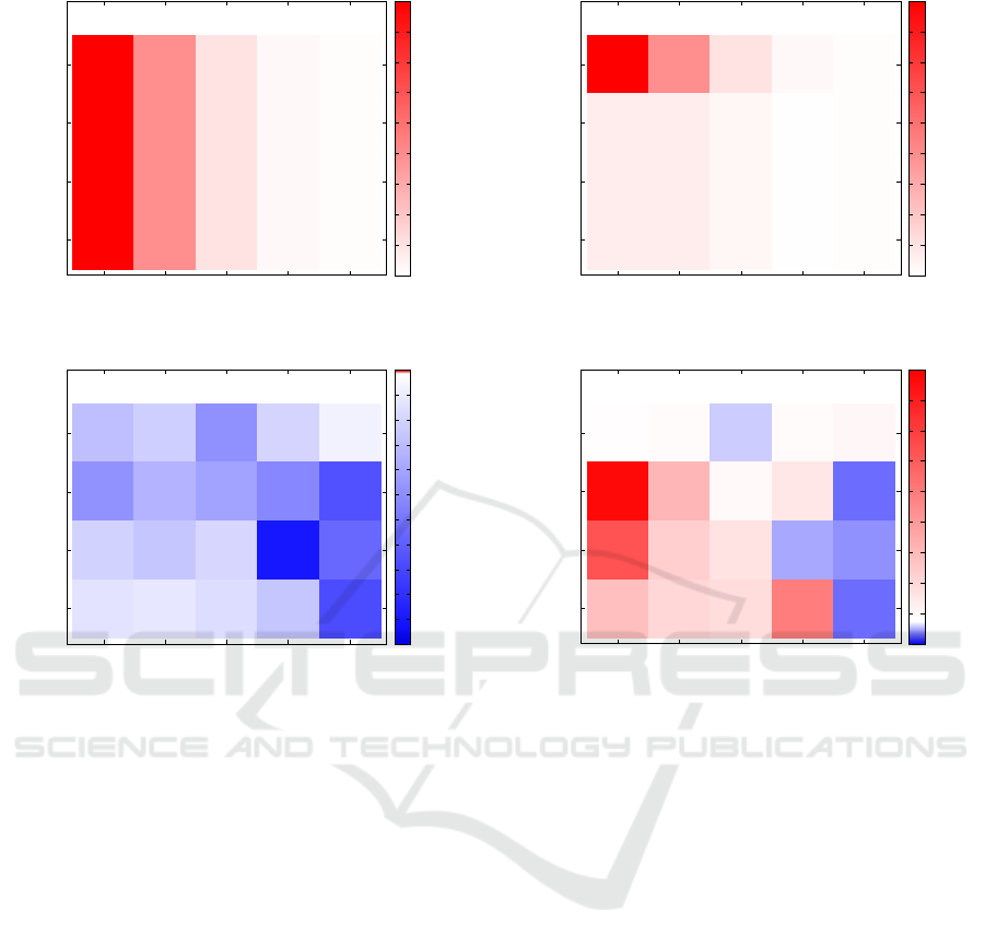
Figure 2 shows the deviation as heat maps for the

two objective functions of the simpliﬁed model. We

observe for this model that all scenarios have a feasi-

ble solution, conﬁrming the beneﬁt from introducing

a mathematical model in the data ﬂow mapping (pre-

liminary experiments carried out with the model used

in (Deng et al., 2016) where the sensors-to-fog map-

ping is based only on the geographic distance were

unable to guarantee feasible solution for high values

of ρ). We observe that, for the ﬁrst objective function,

the deviation is driven just by parameter ρ, which de-

termines the number of fog nodes used by the con-

tinuous model. Indeed, the simpliﬁed model uses all

the available fog nodes, while, especially when ρ is

low, the processing of sensors data may require just

a fraction of the infrastructure computational power,

thus motivating the high value of the deviation.

Focusing, instead, on the second objective func-

tion in Figure 2b, we observe that a higher number

of fog nodes can provide a major reduction in the

response time, as testiﬁed by the large presence of

blue hues in the ﬁgure. A deviation close to -100%

means that the simpliﬁed model halves the average

response time. Indeed, in this case we have an abun-

dance of computational power due to the use of all

the fog nodes, while the continuous model uses just

CLOSER 2020 - 10th International Conference on Cloud Computing and Services Science

258

0.01

0.1

0.1 0.2 0.5 0.8 0.9

δ µ

Obj

Simplified solution divergence [%]

100

200

300

400

500

600

700

800

900

(a) ε(Ob j

)

0.01

0.1

0.1 0.2 0.5 0.8 0.9

δ µ

Obj

Naive solution divergence [%]

-100

-90

-80

-70

-60

-50

-40

-30

-20

-10

(b) ε(Ob j

)

Figure 2: Performance of the Simpliﬁed model.

the minimum amount of resources to satisfy the SLA

constraint.

The performance of the proposed model are

shown in Figure 3. Unlike the previously consid-

ered model, this approach explicitly aims to reduce

the number of fog nodes used. The impact of this

choice is evident in Figure 3a, where we observe a

non-purely vertical pattern in the deviation. Further-

more, we observe that the deviation is, in most of the

cases, much lower compared to the other model – in-

deed the number of fog nodes is is the ceiling value

compared to the value of the CN model. There are a

few noteworthy exceptions, mainly in the case where

the parameter δµ is high. Under these circumstances,

the SLA constraint (13) requires more fog nodes be-

cause using a network link with above than average

delay is likely to result in a SLA violation. Due to the

Boolean nature of the variable E

, a fog node is either

used or not, so the objective function Ob j

reaches

a high value even when ρ is low. The CN model in-

stead allows the use of just a small fraction of every

fog node. This means that the model can use all the

available fog nodes turning them on just for the frac-

0.01

0.1

0.1 0.2 0.5 0.8 0.9

δ µ

Obj

Proposed solution divergence [%]

100

200

300

400

500

600

700

800

900

(a) ε(Ob j

)

0.01

0.1

0.1 0.2 0.5 0.8 0.9

δ µ

Obj2 Naive solution divergence [%]

-100

100

200

300

400

500

600

700

800

(b) ε(Ob j

)

Figure 3: Performance of the proposed model.

tion of their capacity required to satisfy the incoming

load.

Considering the impact of the second objective

function in Figure 3b, we observe that the proposed

model is typically able to achieve performance com-

parable with the continuous model. In some cases

the proposed model outperforms even the continuous

model. To better understand the reasons for this vari-

able performance, we focus on two extreme cases.

For ρ = 0.1 and δµ = 1, the proposed model provides

very poor performance compared to the continuous

alternative. To understand this high response time we

must consider that both the proposed and the contin-

uous models use the same number of fog nodes (just

one). Furthermore, we must factor in the signiﬁcant

impact of network delays (that are not negligible com-

pared to the service time). In this scenario, not being

able to use a fraction of the computational power of

every fog node results in a high impact of the network

delays because we need to make every communica-

tion converge on just one fog node. An opposite case

is when we have a high load and low contribution of

network delays (e.g., ρ = 0.9 and δµ = 0.01). In this

A Location-allocation Model for Fog Computing Infrastructures

259

case, having more fog nodes powered on than what is

strictly necessary (because E

= 1 for all fog nodes)

results in a lower processing time. At the same time,

the low impact of network delays makes the problem

of achieving a good load balancing quite straightfor-

ward because the penalty for reaching a fog node far

away is almost negligible.

4 CONCLUSIONS

In this paper, we focused on a facility location-

allocation problem related to the management of a fog

infrastructure, with special attention to the mapping

of data ﬂows from the sensors to the fog nodes and

from the fog nodes to the cloud data centers. Then,

we propose a mathematical model that starts with a

list of potential fog nodes and selects a minimal sub-

set of them to guarantee the satisfaction of a Service

Level Agreement.

We test the proposed model against alternative

models from the scientiﬁc literature. The experiments

are based on a realistic situation from a project for a

smart city application. We consider a wide range of

scenarios characterized by different load levels and by

different ratios between the service time (that is the

processing time for a set of data from a sensor) and

network delay. The results demonstrate that the pro-

posed model can outperform existing alternatives in

the literature. We also consider an ideal but unreal-

istic model and demonstrate that the proposed model

can, in several cases, achieve a result that is compara-

ble with this ideal solution.

This paper is a step in a wider research line on fog

infrastructure design. We plan to extend our proposal

including quickly and effectively heuristic algorithms

that can be used to solve our problem, and to intro-

duce dynamic scenarios where the load can change

through time.

REFERENCES

Ardagna, D., Ciavotta, M., Lancellotti, R., and Guerriero,

M. (2018). A hierarchical receding horizon algo-

rithm for QoS-driven control of multi-IaaS applica-

tions. IEEE Transactions on Cloud Computing, pages

1–1.

Canali, C. and Lancellotti, R. (2019a). A Fog Computing

Service Placement for Smart Cities based on Genetic

Algorithms. In Proc. of International Conference

on Cloud Computing and Services Science (CLOSER

2019), Heraklion, Greece.

Canali, C. and Lancellotti, R. (2019b). GASP: Genetic Al-

gorithms for Service Placement in fog computing sys-

tems. Algorithms, 12(10).

Cardellini, V., Lo presti, F., Nardelli, M., and Russo russo,

G. (2017). Optimal operator deployment and repli-

cation for elastic distributed data stream processing.

Concurrency Computation, 30(June):1–20.

Celik Turkoglu, D. and Erol Genevois, M. (2019). A com-

parative survey of service facility location problems.

Annals of Operations Research, in press.

Cooper, L. (1963). Location-allocation problems. Opera-

tions Research, 11(3):331–343.

Deng, R., Lu, R., Lai, C., Luan, T. H., and Liang, H. (2016).

Optimal Workload Allocation in Fog-Cloud Comput-

ing Toward Balanced Delay and Power Consumption.

IEEE Internet of Things Journal, 3(6):1171–1181.

Eiselt, H. A. and Laporte, G. (1995). Objectives in location

problems. In Drezner, Z., editor, Facility Location:

A survey of application and methods, pages 151–180.

Springer.

Farahani, R. Z., Fallah, S., Ruiz, R., Hosseini, S., and As-

gari, N. (2019). Or models in urban service facility

location: A critical review of applications and future

developments. European Journal of Operational Re-

search, 276(1):1 – 27.

Khorov, E., Lyakhov, A., Krotov, A., and Guschin, A.

(2015). A survey on IEEE 802.11 ah: An enabling net-

working technology for smart cities. Computer Com-

munications, 58:53–69.

Kramer, R., Cordeau, J.-F., and Iori, M. (2019). Rich vehi-

cle routing with auxiliary depots and anticipated deliv-

eries: An application to pharmaceutical distribution.

Transportation Research Part E: Logistics and Trans-

portation Review, 129:162 – 174.

Marotta, A. and Avallone, S. (2015). A Simulated Anneal-

ing Based Approach for Power Efﬁcient Virtual Ma-

chines Consolidation. In Proc. of 8th International

Conference on Cloud Computing (CLOUD). IEEE.

OpenFog Consortium Architecture Working Group (2017).

OpenFog Reference Architecture for Fog Computing.

Technical report, OpenFog consortium.

Po, L., Rollo, F., Viqueira, J. R., Trillo, R., Lopez, J. C.,

Bigi, A., Paolucci, M., and Nesi, P. (2019). Trafair:

Understanding trafﬁc ﬂow to improve air quality. In

Proc. of IEEE International Smart Cities Conference

(ISC2 2019), Casablanca, Morocco.

Silva, R. A. C. and Fonseca, N. L. S. (2019). On the loca-

tion of fog nodes in fog-cloud infrastructures. Sensors,

19(11).

Yi, S., Li, C., and Li, Q. (2015). A survey of fog comput-

ing: Concepts, applications and issues. In Proceed-

ings of the 2015 Workshop on Mobile Big Data, Mo-

bidata ’15, pages 37–42, New York, NY, USA. ACM.

Yousefpour, A., Ishigaki, G., and Jue, J. P. (2017). Fog

computing: Towards minimizing delay in the internet

of things. In 2017 IEEE International Conference on

Edge Computing (EDGE), pages 17–24.

CLOSER 2020 - 10th International Conference on Cloud Computing and Services Science

260