Product Lifecycle De-trending for Sales Forecasting

Albert F. H. M. Lechner and Steve R. Gunn

School of Electronics and Computer Science, University of Southampton, U.K.

Keywords:

Time Series Prediction, Forecasting, De-trending, ARIMA.

Abstract:

This work introduces a new way to improve the sales forecasting accuracy of time series models using prod-

uct’s life cycle information. Most time series forecasts utilize historic data for forecasting because there is

no data available for the future. The proposed approach should change this process and utilize product life

cycle speciﬁc data to obtain future information including product life cycle changes. Therefore a decision tree

regression was used to predict the shape parameters of the bass curve, which reﬂects a product’s life cycle

over time. This curve is used in a consecutive step to de-trend the time series to exclude the underlying trend

created through the age of a product. The sales forecasts accuracy was increased for all 11 years of a lux-

ury car manufacturer, comparing the newly developed product life cycle de-trending approach to a common

de-trending by differencing approach in a seasonal autoregressive integrated moving average framework.

1 INTRODUCTION

As more data and computational power becomes

available, machine learning is used in many parts of

a manufacturer’s value chain, such as development,

procurement, logistics, production, marketing, sales,

and after-sales, followed by a connected customer af-

ter the purchase (Stock and Seliger, 2016). Analysing

past and current data to improve business is an im-

portant task, but predicting the future is even more

important as several of a company’s decision-making

processes are based on forecasts. Important deci-

sions such as strategic planning, production planning,

sales budgeting, marketing planning or new product

launches are inﬂuenced by forecasts. Therefore, many

practitioners and researchers have focused on new

forecasting methods and improved forecasting accu-

racy as money can be saved and a business’s com-

petitive advantage could be improved (Wright et al.,

1986; Armstrong, 2001).

Machine learning models can outperform tradi-

tional statistical models as they can utilise more fea-

tures of the available data, for that reason companies

use data driven approaches that are able to do so.

Whilst emerging machine learning models increase

accuracy they have challenges and shortcomings from

a practical aspect as they typically have a dense black

box structure which often make them difﬁcult to ex-

plain them within a business environment. It is impor-

tant for businesses to not only increase the accuracy of

a forecast, but also to focus on explainability for the

wider business network. Understanding the main fea-

tures that drive the prediction is not only important for

forecasting but also essential for other departments to

affect the important features and thereby increase fu-

ture sales (Langley and Simon, 1995).

Various techniques are able to model this process,

such as seasonal autoregressive integrated moving av-

erage (SARIMA) models but suffer from drawbacks

being applied on real-world problems. One draw-

back of SARIMA models is that they are not ca-

pable to capture non-linear patterns. For that rea-

son non-linear models were used as well in order to

explain them (Gurnani et al., 2017). To overcome

these problems a new approach was developed based

on a ARIMA model. So far ARIMA models have

not been combined with product life cycle (PLC) de-

trending based on estimated parameters for increased

sales forecasting accuracy as well as increased busi-

ness interpretability.

This work focuses in particular on improving sales

forecasting with the help of machine learning by the

integration of product life-cycle information in tradi-

tional forecasting methods. This approach is of spe-

cial interest in the automotive world, where a car sells

better after its introduction to the market and sells less

over time when newer models from competitors are

introduced, especially when the start of the successor

of the car is already conceivable.

Lechner, A. and Gunn, S.

Product Lifecycle De-trending for Sales Forecasting.

DOI: 10.5220/0009324300250033

In Proceedings of the 5th International Conference on Complexity, Future Information Systems and Risk (COMPLEXIS 2020), pages 25-33

ISBN: 978-989-758-427-5

2 RELATED WORK

Time series forecasting is a frequently researched

topic with many extensions for different special cases.

This topic solves problems in different areas such as

forecasting ﬁnancial markets or sales for a supermar-

ket. For all these cases there are many different mod-

els to choose which have different extensions to their

forecasting capabilities (Montgomery et al., 2008).

Various researchers and practitioners used PLCs to

generate better sales forecasts such as (Solomon et al.,

2000; Hu et al., 2017).

Usually they have a huge number of different

products where individual forecasting is not feasible

for different reasons, therefore they cluster products

into different groups. In order to improve the fore-

casting for new products they use the average PLC

curve sales numbers from clusters that share similar

products. Usually this type of forecasting is used for

products with short PLCs, different to this case where

the life cycle spans over more than seven years. Other

related work uses different data sources in order to

increase the accuracy of monthly car sales forecasts

by including economic variables and Google online

search data (Fantazzini and Toktamysova, 2015). The

previously mentioned approach improves forecasting

but does not include product speciﬁc parameters such

as its age, which will be included in this work.

For statistical models like ARIMA models, there

is no extension to our knowledge that includes a prod-

ucts life cycle into the prediction based on machine

learning estimation of its future sales. For that reason

the following subsection gives an overview about time

series forecasting with a focus on ARIMA models

in Subsection 2.1 as well as an introduction to PLCs

in Subsection 2.2, neural networks in Subsection 2.3,

and decision trees in Subsection 2.4. A combination

of the models named above is then used to create the

new proposed PLC de-trending model in Section 3 to

improve sales forecasts.

2.1 ARIMA Models

Many time series forecasting methods were devel-

oped over the years where the ARIMA model is one

of the most prominent ones. The ARIMA model orig-

inated from the auto regressive moving average mod-

els. Auto regressive refers to the use of past values in

the regression equation for the series; moving average

speciﬁes the error of the model as a linear combina-

tion of error terms that occurred at various times in the

past (Ho et al., 2002). An ARIMA model is described

by its values (p, d, q), where p and q are integers re-

ferring to the order of the auto regressive and moving

average models and d is an integer that refers to the

order of differencing (Zhang, 2003). The equation for

an ARIMA(1, 1, 1) model is given by (Ho et al., 2002)

(1 − φ

B)(1 − B)Y

= (1 − θ

B)ε

(1)

Where φ

is the ﬁrst order auto regressive coefﬁ-

cient and B is a backward shift operator given by

= Y

(t−1)

. The time series at time t is Y

, θ

the ﬁrst order moving average coefﬁcient and ε

is the

random noise at time t (Arunraj and Ahrens, 2015).

The ARIMA model can be used when the time series

is stationary and there is no missing data within the

time series. In the ARIMA analysis, an identiﬁed un-

derlying process is generated based on observations

of a time series to create an accurate model that pre-

cisely illustrates the process-generating mechanism

(Box and Jenkins, 1976). An extension of this model

is the seasonal auto regressive integrated moving av-

erage model, which relies on seasonal lags and differ-

ences to ﬁt the seasonal pattern (Yaffee and McGee,

2009). By including seasonal autoregressive, seasonal

moving average, and seasonal differencing operators

a SARIMA(p, d, q)(P, D, Q)

can be stated as (Arunraj

and Ahrens, 2015)

(B)φ

)(1 − B)

(1 − B

)

c + Θ

(B)Θ

)ε

(2)

where S represents the seasonal length, B the

backward shift operator of a time series observation

lag k symbolized by

= X

t−k

, ϕ

(B) (3)

represents the autoregressive operator of p-order (1 −

(B) − ϕ

) − · ·· − ϕ

)), φ

(B) represents

seasonal autoregressive operator with P-order (1 −

(B) − φ

) − ··· − φ

)), (1 − B)

represents

the differencing operator of order d to remove non-

seasonal stationarity, (1 − B

)

represents the dif-

ferencing operator of order D to remove seasonal

stationarity, c is a constant, Θ

(B) represents the

moving average operator of q-order (1 − Θ

(B) −

)−·· ·− Θ

), and Θ

(B) represents the sea-

sonal moving average operator with Q-order (1 −

(B) − Θ

) − ··· − Θ

)). There are vari-

ous methods for model selection with the most promi-

nent ones Akaike-Information-Criterion (AIC) and

Bayesian-Information-Criterion (BIC). Despite vari-

ous theoretical differences the main difference here is

that BIC penalizes a models complexity more heavily

(Kuha, 2004). The AIC is used for model comparison

in this work and is given by (Kuha, 2004)

AIC(k) = −2

+ 2

(4)

where k is the number of model parameters and

represents the log likelihood, a measure of model ﬁt.

COMPLEXIS 2020 - 5th International Conference on Complexity, Future Information Systems and Risk

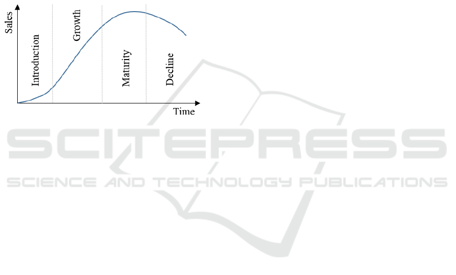
2.2 Product Life Cycle

The new PLC de-trending approach introduced in

Section 3 is based on the PLC that every manufac-

turer’s products go through. Figure 1 depicts this pro-

cess over time. After a product idea goes through

research, development, production, and market roll-

out, it is in the introduction phase. If the product is

successful, sales increase in the second growth phase.

When the product is widely available on the market

and sales stop increasing, the product is in the ma-

turity stage. The demand for the product eventually

declines, and the product reaches its last phase, the

decline stage (Vernon, 1966).

Figure 1: Product life cycle curve.

If the product is successful or the manufacturer

sees it becoming more successful with improvements,

a new product will replace the old one, which restarts

in the ﬁrst phase. The restarts of PLC curves result

in an up and down movement in sales for a partic-

ular product over time. The time frame of a PLC

varies and depends on product, market, and industry

aspects (Meyer, 1997). If a manufacturer produces

more than one product, this information is hard to in-

clude and ﬁlter out in classic time series approaches,

like ARIMA models. For that reason a new approach

was developed in order to include this up and down

generated by different PLCs of all products a com-

pany has on the market. This was initially done by us-

ing neural networks, explained in the following sub-

section.

2.3 Artiﬁcial Neural Networks

Neural networks were chosen as a promising ap-

proach to model the dependencies of the PLC model.

For this reason a short introduction to artiﬁcial neural

networks is given in the following subsection.

One of the most commonly used methods in ML is

artiﬁcial neural networks (ANNs), which try to mimic

the biological brain (Bishop, 1995). The equation for

a simple neural network, the multilayer perceptron, is

given by (Bishop, 1995)

y =

∑

ϕ(w

x + b

) (5)

where w is a vector of weights, x denotes the in-

put vector, b the bias, ϕ is a non-linear activation

function and a are the weights in the output layer.

An ANN consists of several connected nodes, called

neurons, which receive input from other neurons and

send their output to the next neurons. The larger the

network, the more input every neuron receives and

the more neurons in the next layer receive their out-

put (Bishop, 1995). An important feature of ANNs

are that they are nonlinear models as well as univer-

sal approximators that provide competitive results by

using effective training algorithms. Different train-

ing algorithms were used and developed over time:

from back-propagation by (E. Rumelhart et al., 1986)

to newer methods that aim to accelerate the conver-

gence of the algorithm. Although ANNs do not need

any prior assumption to build models, as a model is

mainly determined by the characteristics of the data,

the architecture of the network needs to be predeﬁned

(Haykin, 1994). In 1960, shallow neural networks

with few neurons were used due to the difﬁculty of

training deeper neural networks. More recently, new

techniques have been found to train these networks

and provide state-of-the-art performance. Depend-

ing on the problem, different neural network archi-

tectures evolved over the years. For example, convo-

lutional neural networks are useful for vision prob-

lems (Goodfellow et al., 2016). Over time, many

suitable extensions have been developed, especially

for time series forecasting, such as recurrent neural

networks, which are designed to learn time varying

patterns by using feedback loops (Fausett, 1994). As

from a business perspective the feature importance of

the resulting model is usually very important to ex-

plain the model to stakeholders, other ML techniques

were explored with a focus on decision tree regression

for their better understanding of feature importance,

which are explained in the next subsection.

2.4 Decision Tree Regression

As described in the previous subsection the same

problem of estimating parameters was done using a

decision tree regressor which then was compared to

a neural network. Decision trees have their origin in

machine learning theory and can be used effectively

for classiﬁcation and regression problems. They are

based on a hierarchical decision scheme like a tree

structure. Every tree has a root node followed by in-

ternal nodes that end at one point in terminal nodes.

Each of these nodes takes a binary decision to de-

cide which route to take in the tree until it ends in a

Product Lifecycle De-trending for Sales Forecasting

leaf node. By splitting up a complex problem in sev-

eral binary decisions, a decision tree breaks down the

complexity into several simpler decisions. The result-

ing tree is easier to interpret and understand. Decision

tree regression is a type of a decision tree that approx-

imates real-valued functions. The regression tree is

constructed based on binary recursive partitioning in

an iterative process. All training data is used to se-

lect the structure of the tree. The sum of the squared

deviations from the mean is used to split the data into

parts based on binary splits starting from the top. This

process is continued until a user deﬁned minimum

node size is reached which leads to a terminal node

(Breiman et al., 1984).

This section provided an overview of various tech-

niques used for forecasting. Although different aca-

demics and practitioners use these techniques to im-

prove forecasting, this work identiﬁes a new approach

that improves forecasting accuracy based on the meth-

ods presented. The introduced forecasting methods

range from neural network algorithms to pure time

series methods, like ARIMA models. This new ap-

proach includes model life cycle information in a time

series forecast and is detailed in the following section.

These new ﬁndings support sales and demand fore-

casting for a variety of different businesses.

3 PRODUCT LIFECYCLE

DE-TRENDING

The following section explains how PLC information

can be used to improve sales forecasting (Section 3.1).

The estimation of the Bass curve parameters, that are

used to model the PLC curve is explained further in

Subsection 3.2. The improvements are outlined in

Section 4, based on an application using car sales

data from a luxury car manufacturer in the UK. Im-

plications and future improvements to the proposed

approach are discussed in Section 5.

3.1 Bass Sales De-trending

In the following subsection, a new way to improve

the forecasting accuracy of time series models using

PLC information is introduced. Bringing a product to

market requires a business plan that has to contain not

only an estimated production number over time to jus-

tify ﬁnancial costs but also an estimated time frame

of production until a new product launches (Stark,

2015). Both numbers are based on forecasts and have

limitations, but the important factor is that they tend

to be consistent over time and give a rough estimate

about time and volume of the product. The proposed

approach leverages this information and uses it to de-

trend the time series, consisting of all products of-

fered by the manufacturer. There is no clear deﬁ-

nition of de-trending a time series as there are vari-

ous approaches (Fritts, 1976; Anderson, 1977; Chat-

ﬁeld, 1975). The most common approach is to ﬁt a

straight line to the data and then remove it to yield a

zero-mean residue. Another commonly used proce-

dure is to take the moving mean of the time series and

remove it. This operation needs a pre-deﬁned time

scale, which has little rational basis. Regression anal-

ysis or Fourier-based ﬁltering are examples of more

sophisticated trend extraction methods, which share

the problem of justifying their usage as they are based

on many assumptions (Wu et al., 2007).

Within the new approach, every product needs a

life cycle curve to be ﬁtted based on the expected pro-

duction number and the time frame of production as

well as two shape parameters. By adding all PLC

numbers together, the PLC de-trending curve is cre-

ated and, in a second step, is removed from the sales

time series history. As this information is also avail-

able for a limited time in the future as well, the new

approach adds the lifecycle information to the fore-

cast as well.

There are different ways to ﬁt the PLC curve to

the sales data. In a different approach using the PLC

for new product forecasting, (Hu et al., 2017) used

three different ways to ﬁt a curve to the sales numbers.

They compare piecewise linear curves with polyno-

mial approaches and with the Bass diffusion model

(Bass, 1969). Since their approach clusters the re-

sulting PLC curves, they choose the linear piecewise

over polynomial and Bass curve. However, for this

research, the Bass diffusion model ﬁts the data best

as there are fewer products (ﬁve compared to hun-

dreds) on the market, which have longer life cycles

(7 to 15 years compared to half a year). Piecewise

linear curves as well as polynomial approaches were

explored as well but have not delivered better results

than the Bass curve. Also the estimation of parame-

ters is not as straight forward as from the bass curve

parameter estimation described later in this subsec-

tion. The Bass diffusion curve draws a smooth dif-

fusion curve, including the slow rise of sales in the

beginning and a saturation after the demand increases

over time (Massiani and Gohs, 2016). The Bass diffu-

sion curve is ﬁtted to the available yearly sales num-

bers from 2003 to today. Yearly sales numbers, in-

stead of monthly, were used because of the huge sea-

sonality of car sales, which is not caused by a prod-

uct’s life cycle, but instead is the result of targets

within the business. The seasonality for demand is

much ﬂatter throughout the year as the main impulse

COMPLEXIS 2020 - 5th International Conference on Complexity, Future Information Systems and Risk

for demand is new model introductions, which vary

in time around the world, thus ﬂattening the real de-

mand. There is also seasonality within the demand;

for example, convertibles have higher demand in sum-

mer, but summer varies around the world. The result-

ing Bass curve is then split per month for the pro-

posed approach by converting the sales numbers from

a yearly to a monthly basis, based on the Bass func-

tion. The Bass curve consists of three parameters p, q

and m where m represents the lifetime sales volume

and p and q are shape parameters which representing

the coefﬁcient of innovation and imitation. Therefore,

sales at time T are given by (Bass, 1969)

S(T ) = pm + (q − p)Y (T ) −

[Y (T )]

(6)

Given the yearly sales numbers, the curve was ﬁtted

using a non-linear least squares ﬁtting. As the cars

used for training were already sold m was calculated

by the sum of all past sales. For the years where

no sales numbers were available as a new product

was launching, the Bass curve was calculated using

the parameters predicted by the newly developed ap-

proach later in this subsection. The sales, m, for new

products were calculated using lifecycle business plan

sales numbers (LCBPSN), which are only available to

the business itself. The LCBPSN are used to calculate

the business case of a new car over its entire lifecycle

and are a good approximation of how many cars will

be sold from this model.

Figure 2 depicts the monthly sales numbers in

dark grey as well as the PLC curves ﬁtted with the

Bass diffusion model for two products in blue and or-

ange. The green curve represents the sum of all PLC

curves for 10 years and was used later for division

through the sales numbers to generate a new time se-

ries for forecasting with improved PLC information

PLC de-trended time series =

car sales

∑

bass curves

(7)

3.2 Bass Parameter Estimation

Although the bass curve can be ﬁtted based on as-

sumptions as described above, there is a new way of

estimating the parameters p and q found within this

research. A new approach of ﬁtting the Bass curve

for new products is proposed in the following. By

using sales data from sold products with features like

size and weight it is possible to predict the parameters

of the bass curve for new products by using machine

learning. The data used in this research is a combi-

nation of all car models sales numbers, Bass param-

eters calculated for every model based on past sales

numbers and car speciﬁc features from Car Database

API (Seo and Ltd., 2019) for more than 1000 dif-

ferent car models. The Car Database API features

power, length, width, height, weight, wheelbase and

displacement are numeric and no pre-processing was

necessary; coupe and drive were pre-processed by us-

ing one-hot encoding. In total these features are avail-

able for over 28.000 car models. Yearly sales numbers

are taken from a dataset available within the company

providing the data which consist of all car models sold

since 1990. Out of these sales numbers the Bass pa-

rameters m, p and q were calculated as described in

Subsection 3.1. The following Table 1 shows an ex-

tract from the dataset for two different car models.

The resulting dataset consists of over 1000 differ-

ent car models. The decrease in total car models from

28.000 is due to merging both datasets and remov-

ing entries with missing values. The internal dataset

containing car model sales number only has around

1400 car models whereas the CAR DATABASE API

data lists all cars with different engines separate. This

results in a dataset with no missing values for over

1000 different car models. By ﬁtting a bass curve to

the yearly sales numbers of products already sold, it

is possible to use them as an desired output for the

model. As input, the features of the car models de-

scribed above is used.

For the prediction of p and q a multi regressor ap-

proach using a random forest regressor was compared

to a neural network. The results indicate that the un-

derlying problem can be modelled with a simple neu-

ral network with one hidden layer consisting of 20

neurons. The mean absolute error (MAE) for the neu-

ral network is p = 0.06 and for q = 0.29. These re-

sults were improved by the multi regressor approach

with 100 estimators and a maximal depth of 30 with

an MAE of p = 0.02 and q = 0.11. Also within the

business environment where this model is used, it was

important to get the feature importance for every sin-

gle feature as this information is useful for stakehold-

ers in the business to understand the model and use

the information for the product development of future

cars. As this could be delivered from the linear model

it was the used in the next Section 4. To summarise

the steps from the new PLC approach the following

Table 2 gives a broad overview of all steps. All of

them are conducted on a real world application in the

following section.

4 APPLICATION

The proposed approach of PLC de-trending is pre-

sented for several sales forecasts of the luxury car

Product Lifecycle De-trending for Sales Forecasting

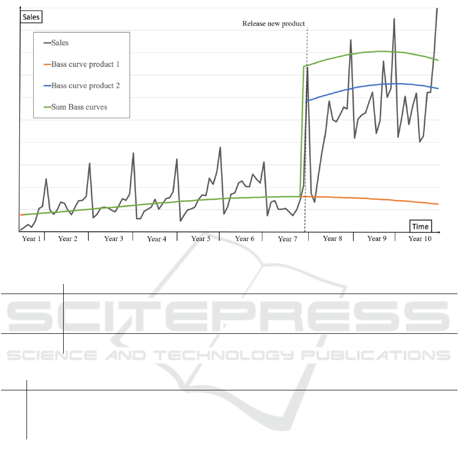
Figure 2: PLC curves for monthly sales data.

Table 1: Data extract for Bass curve ﬁtting.

name year 1 year 2 year 3 year 4 year 5 year 6 year 7 m p q

Suzuki Ertiga 59467 62220 61154 60194 63850 68355 56408 431648 0.055 0.112

Subaru Legacy 219945 280027 244614 244749 228710 198540 187271 1603856 0.089 0.208

name power rpm coupe length width height displacement fuelSystem drive weight

Suzuki Ertiga 105 4500 1 4395 1735 1690 1462 1 2 1180

Subaru Legacy 156 5000 4 4685 1745 1415 2457 2 4 1589

Table 2: PLC algorithm steps.

Step Input Algorithm Output

1. Features of over 1000 cars Decision tree regression p and q for bass curve

2. Companies car model features Decision tree regression from 1. p and q for companies car model

3. p and q from 2. + m from business plan Bass curve PLC curve (cumulated bass curves)

4. Sales time series/ PLC curve from 3. SARIMA model Forecast of PLC de-trended time series

5. Forecast from 4. Multiplication with PLC curve from 3. Final forecast

manufacturer who made the data available with ﬁve

products. The proposed approach outperforms de-

trending by differencing, which is a common ap-

proach to de-trend a time series (Solo, 1984). The

sales data used ranges from May 2003 to December

2018. The forecasts are compared in Table 3 using

the the root mean squared error (RMSE) and MAE for

the years from 2008 to 2018, where the lower error is

highlighted in gray. To build a reasonable SARIMA

model, a minimum of 50 observations was needed,

so more than four years of monthly data were used

(Wei, 1990). To achieve enough input data for the

SARIMA model, only predictions for years after 2007

were considered. The SARIMA model creation it-

self was completed following the classic Box-Jenkins

methodology (Box and Jenkins, 1976).

The models’ hyper parameters p, d, q, P, D, and Q

were chosen from a grid search between zero and

three based on the AIC score. As the business that

generated the sales numbers measures their forecast-

ing accuracy in absolute errors, the MAE was used for

comparison. As the MAE does not penalize huge out-

liers as much as other metrics, the RMSE was used as

well, so both measurements are in the same units as

the forecasted values of car sales. As Figure 2 shows,

the company introduced a new product at the end of

Year 7, which led to an increase in sales. Also, in

2013, 2015, and 2018, new products were released.

Table 3 compares the RMSE and MAE of a classic

SARIMA forecast with de-trending by differencing

COMPLEXIS 2020 - 5th International Conference on Complexity, Future Information Systems and Risk

Table 3: PLC de-trending comparison 2008-2018.

Error\Year 2008 2009 2010 2011 2012 2013 2014 2015 2016 2017 2018

PLC RMSE 30.6 32.7 188.5 57.5 69.1 65.2 56.8 25.9 85.9 76.2 80.9

PLC MAE 22.7 25.1 167.5 49.2 49.7 55.5 50.9 22.1 73.3 68.9 61.7

NDT RMSE 46.1 119.2 2205.2 145.3 124.1 70.9 71.7 46.5 96.8 103.9 192.1

NDT MAE 35.2 77.2 1949.6 117.6 109.7 64.5 62.7 41.9 84.1 89.5 183.6

with the proposed approach, highlighting the lower

error in bold. All years indicate an improvement with

the proposed PLC de-trending approach. For, 2010,

a huge difference is also apparent because it was the

year in which the PLC of one product started with

the introduction of a new product, resulting in higher

sales that were covered within the new approach. In

all 11 years, the new approach resulted in an increased

accuracy for 11 years measured for the MAE as well

as the RMSE.

For all years combined the improvement of the

PLC model for the RMSE is 77% and for the MAE is

78%. Implications for the business were not only in-

creased accuracy in their monthly forecasting, it also

delivered new insights into which features were most

predictive within the decision tree regression and how

they affect shape parameters. Especially newer body

types such as sport utility vehicles have different life

cycle curves compared to traditional sedan models.

They result in a steeper increase at the beginning of

the PLC which was also felt in reality. This informa-

tion can be used for the future planning of new prod-

ucts.

5 CONCLUSIONS

The proposed approach has the advantage of includ-

ing information on PLCs in a sales forecast. Other

methods also include new product information to im-

prove forecast accuracy. However, these methods are

often based on a business’s marketing department’s

forecasts (Kahn, 2002). Hierarchical procedures,

like those proposed by (Lenk and Rao, 1990; Nee-

lamegham and Chintagunta, 1999), use a Bayesian

modelling framework to include various information

sources to make new product forecasts but focus more

on new products than on existing products, unlike the

new PLC approach proposed in this work.

Forecasting every product is also possible, but this

approach has two drawbacks. The ﬁrst one is the lim-

ited amount of historic data for a new product, and

the second one is that new products inﬂuence other

products, so forecasting the total number of sales bet-

ter includes the inﬂuence from a new product onto

other products. In particular, cannibalization from

one product to another product from the same man-

ufacturer is not included, which is an issue that could

further improve the accuracy. As products from other

manufacturers inﬂuence the sales of a product as well,

a general PLC curve containing information about the

life cycles of all products in the same market could

improve forecast accuracy even more. Typically start

and end dates for competitor’s PLCs and their busi-

ness cases are not publicly available, and therefore

including this information was not possible. Other ap-

proaches to ﬁt the PLC curve could be considered as

well, such as extended Bass diffusion models that in-

clude supply constraints, which was not considered so

far (Kumar and Swaminathan, 2003).

Overall sales numbers reﬂected by parameter m

were determined from the business case, which makes

it difﬁcult for people outside of a business to use the

same approach. Therefore an approach which esti-

mated m using a similar approach to the estimation

for p and q was attempted, but the estimate had a large

error which is a consequence of the limited available

data. Further work is required to establish whether the

sales numbers can be estimated reliably from new car

features which would make the approach more widely

applicable. This work would need to explore larger

feature sets as well as suitable modelling approaches.

Although the dataset was using car sales data in the-

ory the approach should work for other products as

well if there is enough data about the features of the

product. As the needed data contains conﬁdential

information it was not possible to get datasets from

other industries and products which could open the

proposed approach to a wider variety of implementa-

tions.

The neural networks accuracy as well as the one

from the decision tree regression could have been im-

proved even further but with that it gets harder to com-

pare both of them. As from a business point the re-

sulting feature importance was more important com-

pared to the accuracy, the decision tree was used. As

the data contains conﬁdential features unique to each

business, it was not possible to get different datasets

the algorithms could be compared and tested on. For

that reason the time series given by the car manufac-

turer was reversed and then forecasted from the oppo-

site side. The results were even better comparing the

Product Lifecycle De-trending for Sales Forecasting

PLC approach to the classic de-trending by differenc-

ing.

Neural networks itself can also be used to fore-

cast time series and not only for modelling the

shape parameters of the bass curve. They are not

well suited for capturing seasonal or trend varia-

tions for unpre-processed data but by de-trending

or de-seasonalization their performance could be in-

creased drastically (Zhang and Qi, 2005). This could

be another approach to change the used SARIMA

model into a neural network model to improve its

accuracy even more with the proposed PLC de-

trending as a pre-processing step for an improved

neural network forecasting model. The problem of

de-seasonalization would not be solved here so this

would need a different pre-processing step.

Although the proposed approach performed better

compared to the current forecasting done by the com-

pany itself there is also room of improvement espe-

cially in how the code is currently executed. Running

the system in a cloud based system would decrease

the time spend running the code with extracting all

the data from different sources. This would allow to

outsource work into the cloud which has proven to

be more efﬁcient for data scientist within a company

(Aulkemeier et al., 2016). This would not only save

time, it could also be run throughout the month more

often in order to get an actual status, live from all re-

gions.

REFERENCES

Anderson, O. D. (1977). The box-jenkins approach to

time series analysis. RAIRO - Operations Research

- Recherche Op

erationnelle, 11(1):3–29.

Armstrong, J. (2001). Principles of Forecasting: A Hand-

book for Researchers and Practitioners. Kluwer.

Arunraj, N. S. and Ahrens, D. (2015). A hybrid sea-

sonal autoregressive integrated moving average and

quantile regression for daily food sales forecast-

ing. International Journal of Production Economics,

170(PA):321–335.

Aulkemeier, F., Daukuls, R., Iacob, M.-E., Boter, J., van

Hillegersberg, J., and de Leeuw, S. (2016). Sales

forecasting as a service. In Proceedings of the 18th

International Conference on Enterprise Information

Systems, ICEIS 2016, page 345–352. SCITEPRESS

- Science and Technology Publications, Lda.

Bass, F. M. (1969). A new product growth for model con-

sumer durables. Management Science, 15(5):215–

227.

Bishop, C. M. (1995). Neural Networks for Pattern Recog-

nition. Oxford University Press, Inc., New York, NY,

USA.

Box, G. E. P. and Jenkins, G. M. (1976). Time series anal-

ysis, forecasting and control. Holden-Day.

Breiman, L., Friedman, J., Olshen, R., and Stone, C. (1984).

Classiﬁcation and regression trees. Routledge, New

York, NY, USA.

Chatﬁeld, C. (1975). The analysis of time series: Theory

and practice. Chapman and Hall.

E. Rumelhart, D., E. Hinton, G., and J. Williams, R. (1986).

Learning representations by back propagating errors.

Nature, 323:533–536.

Fantazzini, D. and Toktamysova, Z. (2015). Forecasting

german car sales using google data and multivariate

models. International Journal of Production Eco-

nomics, 170:97 – 135.

Fausett, L., editor (1994). Fundamentals of Neural Net-

works: Architectures, Algorithms, and Applications.

Prentice-Hall, Inc., Upper Saddle River, NJ, USA.

Fritts, H. (1976). Tree rings and climate. Academic Press.

Goodfellow, I., Bengio, Y., and Courville, A. (2016). Deep

Learning. MIT Press.

Gurnani, M., Korke, Y., Shah, P., Udmale, S., Sambhe, V.,

and Bhirud, S. (2017). Forecasting of sales by using

fusion of machine learning techniques. In 2017 Inter-

national Conference on Data Management, Analytics

and Innovation (ICDMAI), pages 93–101.

Haykin, S. (1994). Neural Networks: A Comprehensive

Foundation. Prentice Hall PTR, USA, 1st edition.

Ho, S. L., Xie, M., and Goh, T. N. (2002). A comparative

study of neural network and box-jenkins arima model-

ing in time series prediction. Comput. Ind. Eng., 42(2-

4):371–375.

Hu, K., Acimovic, J., erize, f., Thomas, D., and

Van Mieghem, J. (2017). Forecasting product life cy-

cle curves: Practical approach and empirical analysis.

Manufacturing & Service Operations Management.

Kahn, K. B. (2002). An exploratory investigation of new

product forecasting practices. Journal of Product In-

novation Management, 19(2):133–143.

Kuha, J. (2004). Aic and bic: Comparisons of assumptions

and performance. Sociological Methods & Research,

33(2):188–229.

Kumar, S. and Swaminathan, J. (2003). Diffusion of innova-

tions under supply constraints. Operations Research,

51:866–879.

Langley, P. and Simon, H. A. (1995). Applications of ma-

chine learning and rule induction. Commun. ACM,

38(11):54–64.

Lenk, P. J. and Rao, A. G. (1990). New models from old:

Forecasting product adoption by hierarchical bayes

procedures. Marketing Science, 9(1):42–53.

Massiani, J. and Gohs, A. (2016). The choice of Bass model

coefﬁcients to forecast diffusion for innovative prod-

ucts: An empirical investigation for new automotive

technologies. Working Papers 2016: 37, Department

of Economics, University of Venice.

Meyer, M. H. (1997). Revitalize your product lines through

continuous platform renewal. Research-Technology

Management, 40(2):17–28.

COMPLEXIS 2020 - 5th International Conference on Complexity, Future Information Systems and Risk

Montgomery, D. C., Jennings, C. L., and Kulahci, M.

(2008). Introduction to Time Series Analysis and Fore-

casting. Wiley.

Neelamegham, R. and Chintagunta, P. (1999). A bayesian

model to forecast new product performance in do-

mestic and international markets. Marketing Science,

18(2):115–136.

Seo and Ltd., W. (2019). Cars technical speciﬁcations

database, https://www.car-database-api.com/.

Solo, V. (1984). The order of differencing in arima models.

Journal of The American Statistical Association - J

AMER STATIST ASSN, 79:916–921.

Solomon, R., Sandborn, P. A., and Pecht, M. G. (2000).

Electronic part life cycle concepts and obsolescence

forecasting. IEEE Transactions on Components and

Packaging Technologies, 23(4):707–717.

Stark, J. (2015). Product Lifecycle Management. Springer.

Stock, T. and Seliger, G. (2016). Opportunities of sustain-

able manufacturing in industry 4.0. Procedia CIRP,

40:536–541.

Vernon, R. (1966). International investment and interna-

tional trade in the product cycle. Quarterly Journal of

Economics, 80:190–207.

Wei, W. (1990). Time Series Analysis: Univariate and Mul-

tivariate Methods. Addison-Wesley Publishing Com-

pany.

Wright, D., Capon, G., Pag

e, R., Quiroga, J., Taseen, A.,

and Tomasini, F. (1986). Evaluation of forecasting

methods for decision support. International Journal

of Forecasting, 2(2):139–152.

Wu, Z., Huang, N. E., Long, S. R., and Peng, C.-K. (2007).

On the trend, detrending, and variability of nonlinear

and nonstationary time series. Proceedings of the Na-

tional Academy of Sciences, 104(38):14889–14894.

Yaffee, R. and McGee, M. (2009). Introduction to time se-

ries analysis and forecasting. Academic Press.

Zhang, P. (2003). Time series forecasting using a hybrid

arima and neural network model. Neurocomputing,

50:159–175.

Zhang, P. and Qi, M. (2005). Neural network forecasting

for seasonal and trend time series. European Journal

of Operational Research, 160:501–514.

Product Lifecycle De-trending for Sales Forecasting