
Objective Measures Ensemble in Associative Classifiers
Maicon Dall’Agnol and Veronica Oliveira de Carvalho
a
Universidade Estadual Paulista (Unesp), Instituto de Geoci
ˆ
encias e Ci
ˆ
encias Exatas, Rio Claro, Brazil
Keywords:
Associative Classifier, Interestingness Measures, Ranking, Classification, Association Rules.
Abstract:
Associative classifiers (ACs) are predictive models built based on association rules (ARs). Model construction
occurs in steps, one of them aimed at sorting and pruning a set of rules. Regarding ordering, usually objective
measures (OMs) are used to rank the rules. The aim of this work is exactly sorting. In the proposals found
in the literature, the OMs are generally explored separately. The only work that explores the aggregation of
measures in the context of ACs is (Silva and Carvalho, 2018), where multiple OMs are considered at the same
time. To do so, (Silva and Carvalho, 2018) use the aggregation solution proposed by (Bouker et al., 2014).
However, although there are many works in the context of ARs that investigate the aggregate use of OMs, all
of them have some bias. Thus, this work aims to evaluate the aggregation of measures in the context of ACs
considering another perspective, that of an ensemble of classifiers.
1 INTRODUCTION
Right now, people are generating and storing data.
This huge amount of data stores valuable information
that companies can use to better understand their cus-
tomers, improve their budgets, and so on. For this,
it is important to use techniques that automatically
discover interesting patterns in the domain. Classifi-
cation and association rules (ARs) are among these
techniques. Associative Classifiers (ACs) are rule-
based classifiers that are built using association rules.
ACs have the advantage of exploring the search space
in a broader view, compared to, for example, C4.5,
which does a greedy search. AC yields good re-
sults compared to other machine learning algorithms
(Yang and Cui, 2015; Abdellatif et al., 2018b), espe-
cially decision trees, rule induction and probabilistic
approaches (Abdellatif et al., 2018a). According to
(Yang and Cui, 2015), one of the main advantages of
ACs is that the output is represented in simple if-then
rules, making it interpretable for the end-user. Be-
sides, according to (Kannan, 2010) ACs naturally deal
with missing values and outliers, as they only manip-
ulate statistically significant associations and ensure
that no assumption is made about attribute depen-
dence or independence. Some domain applications
that use ACs can be seen in (Nandhini et al., 2015;
Singh et al., 2016; Moreno et al., 2016; Shao et al.,
2017; Alwidian et al., 2018; Yin et al., 2018).
a
https://orcid.org/0000-0003-1741-1618
Many ACs exist, as seen in (Thabtah, 2007; Abdel-
hamid and Thabtah, 2014), which provide a good re-
view of the topic. The first and generally the one used
as baseline in the literature works is CBA (Liu et al.,
1998). In general, three steps are necessary to build an
AC: (a) extraction of a set of association rules where
the consequents contains only labels; (b) model build-
ing through sorting and pruning; (c) prediction. ACs
algorithms differ in how they perform each step, es-
pecially steps (b) and (c). Regarding step (b), one
way to sort the rules to choose which ones will be
in the model is through objective measures (OMs).
Step (b) is important because many rules can be ex-
tracted from step (a) and, in general, many of them
are not relevant to the model. Therefore, an efficient
evaluation of ARs is an essential need (Yang and Cui,
2015; Abdellatif et al., 2019). This work contributes
to step (b). According to (Abdelhamid et al., 2016),
one of the challenges related to ACs is sorting, be-
cause choosing the appropriate ranking criterion is a
critical task that impacts the accuracy of the classifier.
In the proposals found in the literature, OMs
are generally explored separately in ACs (see Sec-
tion 2.3). The only work that explores the aggre-
gation of measures in the context of ACs is (Silva
and Carvalho, 2018), where multiple OMs are con-
sidered at the same time. To do so, (Silva and Car-
valho, 2018) use the aggregation solution proposed
by (Bouker et al., 2014). However, although there are
many works in the context of ARs that investigate the
aggregate use of OMs (see Section 2.2), all of them
Dall’Agnol, M. and Oliveira de Carvalho, V.
Objective Measures Ensemble in Associative Classifiers.
DOI: 10.5220/0009321600830090
In Proceedings of the 22nd International Conference on Enterprise Information Systems (ICEIS 2020) - Volume 1, pages 83-90
ISBN: 978-989-758-423-7
Copyright
c
2020 by SCITEPRESS – Science and Technology Publications, Lda. All rights reserved
83

have some bias.
Considering the above, this work aims to evalu-
ate the aggregation of measures in the context of ACs
considering another perspective, that of an ensemble
of classifiers. Ensemble classifiers, such as random
forest, build several classifiers and then combine their
classifications to decide to which class label a given
object belongs to. Using this idea it is possible to
consider many OMs at the same time, each of them
generating an AC that can be combined later. Good
results were obtained compared to those presented by
(Silva and Carvalho, 2018), indicating that an ensem-
ble of OMs ACs can be a suitable solution.
This work is structured as follows: Section 2 re-
views some concepts and discusses related works.
Section 3 describes the ensemble approach, which is
followed by experiments (Section 4), results and dis-
cussion (Section 5). Section 6 concludes the paper
with conclusions and future works.
2 REVIEW AND RELATED
WORKS
This section presents some concepts needed to under-
stand the current work (Section 2.1), as well, some
related works (Section 2.3) and approaches used to
aggregate OMs (Section 2.2).
2.1 Associative Classifier
An associative classifier (AC) aims to obtain a predic-
tive model based on a process that uses class associa-
tion rules (CARs). A class association rule A ⇒ c is
a special case of an association rule in which the con-
sequent only contains a class label. Formally, given
D a dataset containing a set of items I = {i
1
, ..., i
n
}, a
set of class labels R = {c
1
, ..., c
p
} and a set of trans-
actions T = {t
1
, ...,t
m
}, where each transaction t
i
∈ T
contains a subset of items A ⊆ I and one class label
c ∈ R such that t
i
= A ∪c. A class association rule is a
relation A ⇒ c, in which A ⊆ I and c ∈ R. Rule A ⇒ c
occurs in the set of transactions T with confidence
con f and support sup, where P(Ac) represents rule
support (probability of A ∪ c occurrence) and P(c|A)
rule confidence (conditional probability of c given A).
In this context, items in I are usually <attribute,
value> pairs, because CARs are extracted from re-
lational tables containing m objects (instances) de-
scribed by k attributes (features), where each object
O
i
is associated with one of the p known class la-
bels to be predicted. Each object O
i
is, therefore, de-
scribed by a vector O
i
= [v
i1
, v
i2
, ..., v
ik
, c
i
], where v
i j
is a <attribute, value> pair representing the value of
object i in attribute j and c
i
the class label associated
with O
i
.
As mentioned in the introduction, among the
many ACs algorithms, CBA (Liu et al., 1998) is gen-
erally the most commonly used as baseline. Briefly,
the algorithm works as follows: first a set of CARs is
obtained (step (a)). After that, CARs are sorted ac-
cording to three criteria: confidence, support and or-
der of generation. Based on these criteria, a rule r
i
precedes a rule r
j
, in a sorted list, if confidence(r
i
)
> confidence(r
j
); if the confidences are the same, but
support(r
i
) > support(r
j
); if the supports are the same,
but r
i
was generated before r
j
. This is where this work
contributes. Considering this sorting pruning occurs.
For each rule r it is checked the transactions it cov-
ers and if it correctly covers at least one transaction.
In this case, the rule is selected to be included in the
model and all transactions covered by it are removed
from the dataset. Pruning completes step (b). Regard-
ing step (c), given an unseen object, the class label as-
sociated with the first rule that matches the object is
the one to which it will be classified.
As can be observed, sorting affects the whole pro-
cess. It is based on the sorted rule list that pruning is
performed. Therefore, depending on the criteria used
in sorting a different classifier is obtained.
2.2 Aggregation Approaches
A common way used by ACs algorithms to sort the
rules in step (b) is through objective measures, as sup-
port and confidence. An OM is used to compute a
value that express the relevance of a rule by only con-
sidering the information available in the dataset. Gen-
erally, the higher the value the better the rule. Based
on these values, it is possible to create a sorted rule
list. 61 OMs are defined and discussed in (Tew et al.,
2014), presenting a good review on the topic; there-
fore, these measures are not described here.
As many OMs exist, solutions have been proposed
to help the user to decide which one to choose/use. A
review discussing some of these solutions can be seen
in (Bong et al., 2014). Among them there are some
solutions that aim to aggregate the values of two or
more OMs so that the user does not have to select a
specific one to order the rules as in (Nguyen Le et al.,
2009) and (Yang et al., 2009). The first uses Choquet
Integral to aggregate, while the second uses genetic
network programming (GNP) to solve the problem,
being necessary to set several parameters that influ-
ence the results.
(Bouker et al., 2014) propose an aggregation solu-
tion that, because it is deterministic and based solely
on the information contained in the data, was chosen
ICEIS 2020 - 22nd International Conference on Enterprise Information Systems
84

for use in the work of (Silva and Carvalho, 2018).
There are other works based on the same ideas of
(Bouker et al., 2014) as that of (Dahbi et al., 2016).
To sort rules, (Bouker et al., 2014) use the concept of
rule dominance. It is defined that a rule r
i
dominates a
rule r
j
(r
i
r
j
) when all OMs values in r
i
are greater
than or equal to the OMs values in r
j
– if the values
are all the same, the rules are considered equivalent,
i.e., to have dominance, the value of at least one mea-
sure must be greater. Comparisons where there is no
dominance of one of the rules, they are considered as
undominated among themselves.
To get the sorted list, an algorithm called SkyRule
is executed iteratively, which returns at each execu-
tion a set of undominated rules, i.e., a set of rules that
are not dominated by any other rule. The SkyRule
algorithm is loop-based, so that at each iteration the
rules most similar to the reference rule (r
⊥
) that are
also undominated are extracted. These rules are called
r
∗
. Similarity is computed through normalized Man-
hattan distance, i.e., through the arithmetic mean of
the normalized differences. The reference rule rep-
resents the aggregation of the computed OMs for all
rules, storing the best value obtained for each OM in
the rule set. The rules returned by SkyRule are added
to a E
i
set and removed from the rule set (i indicates
the interaction in which the rules were extracted). The
process repeats until the rule set be empty. At the end
of the process there is a set of sets that make up the
sorting. Note that the idea is that less dominated rules
are considered better.
Table 1: Example of some rules evaluated by some mea-
sures. Adapted from (Bouker et al., 2014).
Rule OM-1 OM-2 OM-3
r
1
0.2 0.67 0.02
r
2
0.1 0.50 0.00
r
3
0.1 0.50 0.02
r
4
0.2 0.40 0.10
r
5
0.2 0.33 0.02
r
6
0.2 0.33 0.10
r
7
0.1 0.20 0.01
r
8
0.1 0.17 0.02
Consider, for example, 8 rules evaluated by 3 OMs,
as seen in Table 1. Here, r
⊥
={0.20, 0.67, 0.10}. In
the first iteration of the first SkyRule execution r
1
is
the first rule to be considered as r
∗
(the most similar
to r
⊥
); therefore, it is added in the return set. Since
r
1
dominates r
2
, r
3
, r
5
, r
7
and r
8
, they are discard
form this SkyRule execution, remaining only r
4
and
r
6
. Next, r
4
is chosen as r
∗
and is also added in the
return set, which removes r
6
from the current execu-
tion, finishing the search for undominated rules. Af-
ter the first SkyRule execution, E
1
= {r
1
, r
4
}. These
rules are removed from the original rule set and, in
the next iteration, SkyRule is executed without con-
sidering them, which in turn results in E
2
= {r
3
, r
6
}.
Repeating the process it is obtained in the third itera-
tion E
3
= {r
5
, r
2
} and in the fourth E
4
= {r
7
, r
8
}, thus
establishing the sorting of the 8 rules. Finally, to visu-
alize the results obtained through the ranking process,
it is possible to build a graph showing the sequence
of creation of the sets, as seen in Figure 1. Therefore,
the final ranking is as follows: r
1
, r
4
, r
3
, r
6
, r
2
, r
5
, r
7
and r
8
.
Figure 1: Visualization of the sequence of creation of the
sets used to sort the rules presented in Table 1. Adpated
from (Bouker et al., 2014).
Finally, it is important to mention that if there is more
than one rule in the same E
p
set, a tiebreaker is per-
formed by similarity of the rules to the reference rule
– the most similar ones are ranked first. In cases
where there are still ties, the tie is broken by order
of generation, giving preference to the rules that were
first generated, as in CBA.
2.3 Related Works
Although there is much work on associative classifi-
cation, few explore the effect of OMs on the sorting
process. (Azevedo and Jorge, 2007) explore the use of
10 OMs in 17 datasets regarding sorting and predic-
tion in ACs and conclude that Conviction is the most
appropriate OM to be used.
(Jalali-Heravi and Za
¨
ıane, 2010) assess the impact
of 53 OMs on each phase of the ACs construction
(steps (a), (b) and (c)). Regarding step (b) the au-
thors explore the sorting with and without pruning.
Regarding step (c) the authors explore two strategies:
(i) select the best ranked rule that covers the instance
and (ii) divide all the rules that cover the instance into
groups, according to the class label, and perform the
average of the values of the OM in analysis in each
group; in this case, the group with the best average
Objective Measures Ensemble in Associative Classifiers
85
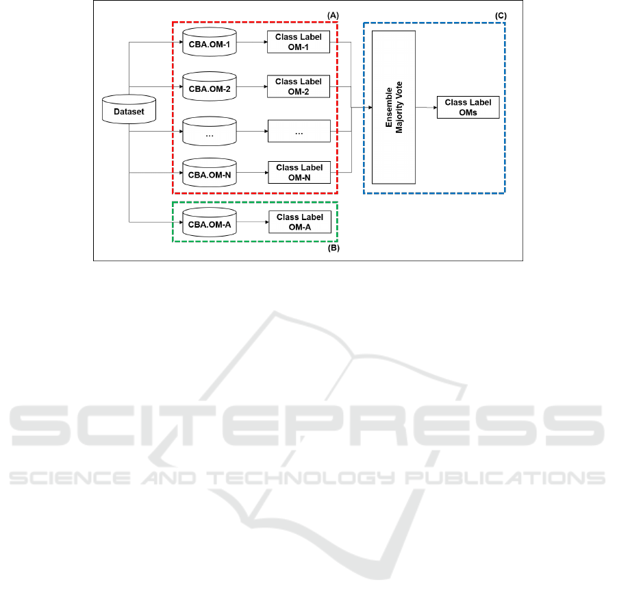
Figure 2: Ranking views: individual, aggregate and ensemble.
defines the class label. Regarding the sorting crite-
ria, the following precedences are used: value of the
measure being analyzed, support and rule size (gen-
eral rules are preferred over the specific ones). The
analysis is done on 20 datasets. The authors conclude
that many of the analyzed OMs improve classifier per-
formance. However, there is no measure that is best
suited for all datasets or for all classifier steps.
(Kannan, 2010) assess the influence of 39 OMs on
pruning and sorting. The authors test 3 sorting alter-
natives: (i) only a given measure, (ii) a given measure
plus tiebreaker criteria, as in CBA (confidence, sup-
port, and rule generated first) and (iii) sorting by a
given measure, followed by reordering, through strat-
egy (ii), of the best k rules selected. The study was
conducted on a single dataset for students from a dis-
tance learning program. The authors conclude that
AC accuracy can be improved by using appropriate
OM for pruning and ordering.
(Yang and Cui, 2015) aim to improve the perfor-
mance of ACs in unbalanced datasets by studying 55
OMs in 9 datasets. The authors point out that this is a
relevant problem, as OMs can be applied in different
steps, such as rule generation, pruning and sorting.
Two types of analysis are performed: (i) one to find
similar OMs groups in unbalanced datasets; (ii) the
other to identify the most appropriate OMs to be used
in the presented context. With respect to (i), the au-
thors use graph-based clustering as well as frequent
pattern mining. Regarding (ii), the authors use CBA
to compute its performance, via AUC (area under the
ROC curve), when sorting is performed by each of the
OMs individually. In conclusion, it is suggested to use
26 OMs divided into two groups: one focused on ex-
tremely unbalanced datasets and the other focused on
slightly unbalanced datasets.
Unlike the above works, (Silva and Carvalho,
2018) explore the aggregation of OMs in the con-
text of ACs, where multiple OMs are considered at
the same time. To do so, they used the aggregation
solution proposed by (Bouker et al., 2014) (see Sec-
tion 2.2). To this end, the authors modified step (b)
of CBA, specifically sorting, as follows: a rule r
i
pre-
cedes a rule r
j
, in a sorted list, if the aggregated OMs
values in r
i
are greater than r
j
; in the event of a tie, r
i
was generated before r
j
. In other words, the sorting
follows the list generated by applying (Bouker et al.,
2014) approach. The authors noted that aggregation
tends to improve the accuracy of ACs, compared to
the use of individual OMs, as done in other works.
However, aggregation approaches may present some
problems, as discussed below (Section 3).
3 ENSEMBLE APPROACH
It can be seen from the works of Section 2.3 that the
problem presented here is relevant, since the most
modifiable CBA step is that of sorting, as it can be
done using many OMs; the other steps have more pre-
defined procedures. The revised works can be basi-
cally divided into two views, as shown in Figure 2:
those that explore the OMs individually (view (A) in
red) and those that explore the OMs at the same time
(view (B) in green). In the latter case, only one was
found. Unlike the literature, this current work intends
to explore the problem from another perspective, that
of an ensemble of classifiers (view (C) in blue). As
noted by (Silva and Carvalho, 2018), aggregate mea-
sures provide, on average, better results. The ensem-
ICEIS 2020 - 22nd International Conference on Enterprise Information Systems
86

ble view has the advantage of using many OMs at the
same time, regardless of which one is best suited for a
given dataset, which is what happens in the individual
view. However, in general, aggregation approaches
have some bias that generates problems, such as the
one presented in (Bouker et al., 2014) and used by
(Silva and Carvalho, 2018).
In works that use the concept of dominance, such
as (Bouker et al., 2014) and (Dahbi et al., 2016),
the greater the number of OMs to be aggregated the
greater the likelihood that an OM will cause a rule r
to be undominated. This fact only generates a com-
plete set of undominated rules, resulting in only one
iteration of RankRule. That is, a single E
p
containing
all the rules is obtained. In this way, the final sort-
ing is done, in fact, only by the similarity of the rules
in relation to the reference rule, or even, in case of
a tie, by the rule ID (generated first), thus losing the
purpose of searching by undominated rules. As men-
tioned before, similarity is computed through normal-
ized Manhattan distance, i.e., through the arithmetic
mean of the normalized differences.
For a better understanding of the problem, con-
sider two rules associated with 10 OMs: OMs
r
i
={0.9,
0.98, 0.89, 0.88, 0.95, 0.99, 0,79, 0.8, 0.79, 0.96}
and OMs
r
j
={0.1, 0.10, 0.08, 0.20, 0.11, 0.03, 0, 0.3,
0.15, 0.98}. It is remarkable that r
i
is better than r
j
in almost all values; however, because measure 10 in
OMs
r
j
is greater than measure 10 in OMs
r
i
(0.98 x
0.96), there would be no dominance between them
and therefore both would belong to the same E
p
set.
Expanding to a set of more rules and more OMs, the
problem begins to get worse, because if a measure in
one rule is greater than in another rule, the problem
will occur.
Due to the above problems, the focus here is to
assess the impact of using many OMs at the same time
considering an ensemble of classifiers. Thus, as seen
in Figure 2, the process works as follows:
i. Generate an individual classifier for each OM. To
this end, step (b) of CBA is modified, specifically
sorting, as follows: a rule r
i
precedes a rule r
j
,
in a sorted list, if the individual OM value in r
i
is
greater than r
j
; in the event of a tie, r
i
was gener-
ated before r
j
;
ii. Label the new unseen object by each individual
OM classifier and then realize a majority vote to
decide the class label to which the instance will
belong. In case of a tie, the majority class associ-
ated with the dataset is considered.
4 EXPERIMENTAL EVALUATION
Experiments were performed to evaluate the proposed
approach. For this, the necessary requirements for the
experiments are presented. The proposed approach
was compared with those found in the literature, as
shown in Figure 2: individual OMs (view (A)) and
aggregate OMs (view (B)). Note that the aggregation
approach to be used could be any other available in
the literature. However, it was chosen to use (Bouker
et al., 2014) approach as it was the one used by (Silva
and Carvalho, 2018). Future work intends to expand
the analysis to include other aggregation approaches
in order to make a broader comparison with the en-
semble approach proposed here. Finally, it was cho-
sen to use the same settings used by (Silva and Car-
valho, 2018) to make a fair comparison.
Datasets. 8 datasets available in UCI
1
were used,
which are presented in Table 2 – in the total num-
ber of features the identification columns are being
disregarded and the one associated with the class la-
bels is considered. Discretization was performed by
the algorithm proposed by (Fayyad and Irani, 1993)
available in Weka
2
. Data were preprocessed to fit the
datasets to the input format used in the CBA imple-
mentation adopted here (available in (Coenen, 2004)).
Missing values and features without distinct values af-
ter discretization were ignored.
Table 2: Datasets used in experiments: Australian Credit
Approval (Australian); Breast Cancer Wisconsin (Breast-
C-W); Glass Identification (Glass); Heart; Iris; Tic-Tac-
Toe; Wine; Vehicle Silhouettes (Vehicle). Acronyms mean:
#Transactions (#T); #Features (#F); #Distinct Items (#D-I);
#Class Labels (#C-L).
Dataset #T #F #D-I #C-L
Australian 690 15 51 2
Breast-C-W 699 10 38 2
Glass 241 10 29 7
Heart 270 14 30 2
Iris 150 5 17 3
Tic-Tac-Toe 958 10 29 2
Wine 178 14 41 3
Vehicle 946 19 36 4
Objective Measures. 19 OMs were considered: Sup-
port, Prevalence, K-Measure, Least Contradiction,
Confidence, EII1, Leverage, DIR, Certainty Factor,
Odds Ratio, Dilated Q2, Added Value, Cosine, Lift, J-
Measure, Recall, Specificity, Conditional Entropy and
1
https://archive.ics.uci.edu/ml.
2
https://www.cs.waikato.ac.nz/ml/weka/.
Objective Measures Ensemble in Associative Classifiers
87

Coverage. This choice was made based on the work
of (Tew et al., 2014), as described in (Silva and Car-
valho, 2018).
Parameters Setting. Minimum support and mini-
mum confidence were set, respectively, to 5% and
50%. The values were empirically defined. In addi-
tion, the following limits were considered in the im-
plementation of CBA used here (available in (Coenen,
2004)): (i) maximum amount of antecedent items: 6;
(ii) maximum amount of frequent itemsets to be ob-
tained: 5.000.000; (iii) maximum amount of rules to
be extracted: 10.000.
Evaluation Criterion. Accuracy was used as a
measure of performance. For this, a 10-fold strati-
fied cross-validation was performed 10 times. There-
fore, the accuracy values presented here represent the
average of 10 runs. Aiming at the fairness of the re-
sults, the same training and testing sets were used for
a given i iteration in each of the 10 times the 10-fold
stratified cross-validation was performed, i.e., in all
configurations, in the nth iteration, the training and
test sets were the same.
Experimental Configuration Overview. Each
dataset was executed in 22 different configurations,
as follows: (1
◦
) CBA, (2
◦
) Support, (3
◦
) Prevalence,
(4
◦
) K-Measure, (5
◦
) Least Contradiction, (6
◦
)
Confidence, (7
◦
) EII1, (8
◦
) Leverage, (9
◦
) DIR,
(10
◦
) Certainty Factor, (11
◦
) Odds Ratio, (12
◦
)
Dilated Q2, (13
◦
) Added Value, (14
◦
) Cosine, (15
◦
)
Lift, (16
◦
) J-Measure, (17
◦
) Recall, (18
◦
) Speci-
ficity, (19
◦
) Conditional Entropy, (20
◦
) Coverage,
(21
◦
) OMs.Aggregate (OMs.A) and (22
◦
) Ensemble
(OMs.E). Number “1” refers to CBA without any
modification; Number “2” to “20” to CBA modified
to sort the rules according to a specific OM (indi-
vidual OMs (view (A) in Figure 2)); Number “21”
to CBA modified to sort the rules according to the
aggregate approach proposed by (Bouker et al., 2014)
(aggregate OMs (view (B) in Figure 2)); Number
“22” to the ensemble approach presented here (view
(C) in Figure 2). Note that these “22” configurations
cover the three views presented in Figure 2.
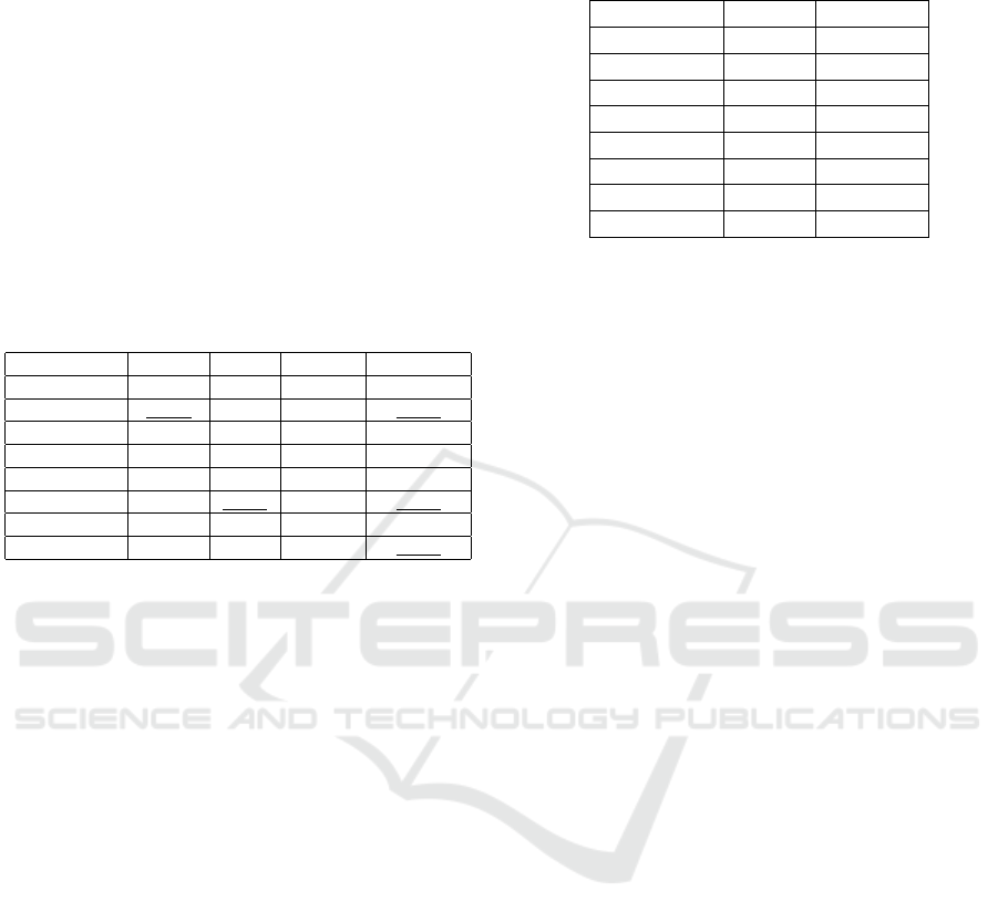
5 RESULTS AND DISCUSSION
To better understand the results the analysis was di-
vided considering different views. The first, shown in
Table 3, compares the obtained accuracies in the En-
semble approach (OMs.E) with CBA. The best value
obtained in each dataset is highlighted. For example,
considering the Australian dataset, the best accuracy
(86.58%) occurred in the Ensemble approach. Note
that OMs.E performs better on 5 datasets (62.50%),
providing a good solution, as each OM in the ensem-
ble evaluates each rule in a different way. The sec-
ond, shown in Table 4, compares the obtained accu-
racies in the Ensemble approach with the aggregate
approach proposed by (Bouker et al., 2014) (OMs.A).
The best value obtained in each dataset is highlighted.
It can be seen that OMs.E perform better on 4 datasets
(50.0%), tying with OMs.A (50.0%). Also, as men-
tioned in Section 3, as many OMs are used in the
(Bouker et al., 2014) approach, the final sorting is
done, in fact, only by the similarity of the rules in
relation to the reference rule. In all cases here, only
one E
p
set was generated (E
p
= 1), which means that
a simple similarity yields good results and no search
for undominated rules is required, as the process can
be simplified. Future work intends to use these results
to propose another aggregation approach.
Table 3: Comparison of results between CBA and Ensem-
ble.
Dataset CBA Ensemble
Australian 86.04 86.58
Breast-C-W 96.07 95.95
Glass 64.85 65.14
Heart 80.67 82.19
Iris 95.67 96.00
Tic-Tac-Toe 100.00 98.59
Wine 98.87 95.11
Vehicle 58.76 59.07
Table 4: Comparison of results between Ensemble and
OMs.A.
Dataset Ensemble OMs.A
Australian 86.58 85.17
Breast-C-W 95.95 93.71
Glass 65.14 66.23
Heart 82.19 83.15
Iris 96.00 97.07
Tic-Tac-Toe 98.59 90.40
Wine 95.11 98.87
Vehicle 59.07 58.26
Evaluating the results in a general view, the obtained
accuracies among CBA, OM (view (A) in Figure 2),
OMs.A (view (B) in Figure 2) and Ensemble (view
(C) in Figure 2) were compared, as shown in Ta-
ble 5. The OM column presents the best accuracy
obtained among the 19 OMs used in the experiments
(the name(s) of the OM(s), regarding each value,
ICEIS 2020 - 22nd International Conference on Enterprise Information Systems
88
is(are) mentioned on the figure label). The best value
obtained in each dataset is highlighted. It can be noted
that:
• CBA performs best on 2 datasets (25%, counting
the tie), OM at 2 (25%), OMs.A at 4 (50%, count-
ing the tie) and OMs.E at 1 (12.50%). As seen,
solutions that use multiple OMs perform better
than individual OMs, in this case 62.50% (5 oc-
currence).
Table 5: Comparison of results among CBA, OM, OMs.A
and Ensemble. *Best OMs accuracies: Australian: Added
Value; Breast-C-W: J-Measure; Glass: J-Measure, Odds
Ratio; Heart: J-Measure; Iris: Dilated Q2; Tic-Tac-Toe:
Odds Ratio, Confidence; Wine: J-Measure; Vehicle: K-
Measure.
Dataset CBA OM* OMs.A Ensemble
Australian 86.04 86.29 85.17 86.58
Breast-C-W 96.07 96.32 93.71 95.95
Glass 64.85 66.08 66.23 65.14
Heart 80.67 82.93 83.15 82.19
Iris 95.67 96.07 97.07 96.00
Tic-Tac-Toe 100.00 99.99 90.40 98.59
Wine 98.87* 96.94 98.87* 95.11
Vehicle 58.76 61.89 58.26 59.07
• Looking at cases where the Ensemble approach
does not have the best values, such as those pre-
sented in Table 4, where OMs.A wins, it is inter-
esting to note that in two of them (Breast-C-W and
Vehicle) it loses to the best OM, which is a good
result, as it performs close to the best OM. This
means that Ensemble is incorporating its effect in
the result. This is why their values are underlined.
In the latter case (Tic-Tac-Toe), although CBA
presents the best performance, the same pattern
occurs, i.e., it performs close to the best OM (un-
derlined value). Considering this, Ensemble wins
4 times (50.0%) and OMs.A 4 (50.0%), as already
shown in Table 4. In addition, Table 6 comple-
ments Table 5 by presenting the differences be-
tween OMs.A and Ensemble with respect to the
best accuracy observed in each dataset. The high-
lighted values correspond to the smallest differ-
ence between the best accuracy and the respective
setting. As seen, Ensemble wins 4 times (50.0%)
and OMs.A 4 (50.0%), with differences in Ensem-
ble smaller than OMs.A (an average of 1.44 vs
2.16).
• Only 6 OMs appeared in Table 5, which means
that 13 of 19 did not show good values in any of
the datasets. These OMs may be negatively influ-
encing the accuracy of solutions that use multiple
OMs. Therefore, an in-depth study of the most
appropriate OMs to be aggregated into the pre-
Table 6: Differences between OMs.A and Ensemble regard-
ing the best accuracy observed in each dataset.
Dataset OMs.A Ensemble
Australian 1.41 0.00
Breast-C-W 2.61 0.37
Glass 0.00 1.09
Heart 0.00 0.96
Iris 0.00 1.07
Tic-Tac-Toe 9.60 1.41
Wine 0.00 3.76
Vehicle 3.63 2.82
sented approaches (aggregate, ensemble) should
be undertaken.
6 CONCLUSIONS
This work presented an ensemble solution to consider
many OMs, at the same time, in the sort step of CBA
to improve its accuracy. According to the obtained
results, it was noted that solutions that use multiple
OMs perform better than individual OMs. Regarding
the Ensemble approach, it was found to be a good so-
lution, especially when the best accuracy is related
to the best OM. However, the Ensemble approach
achieved the same performance as OMs.A, each win-
ning 50% of the times. Thus, both presented them-
selves as good solutions, each one better in one spe-
cific situation, even OMs.A having the bias previously
explained.
In order to improve results as well as analyzes, fu-
ture works should be done: (i) consider more datasets;
(ii) explore other aggregation approaches beyond that
considered here (Bouker et al., 2014); (iii) find ways
to automatically select the most appropriate OMs to
be aggregated in the presented approaches (aggre-
gated, ensemble).
ACKNOWLEDGEMENTS
We wish to thank Fapesp, process number
2019/04923-2, for the financial aid.
REFERENCES
Abdelhamid, N., Jabbar, A. A., and Thabtah, F. (2016). As-
sociative classification common research challenges.
In 45th International Conference on Parallel Process-
ing Workshops, pages 432–437.
Abdelhamid, N. and Thabtah, F. A. (2014). Associative
classification approaches: Review and comparison.
Objective Measures Ensemble in Associative Classifiers
89

Journal of Information & Knowledge Management,
13(3).
Abdellatif, S., Ben Hassine, M. A., and Ben Yahia, S.
(2019). Novel interestingness measures for mining
significant association rules from imbalanced data. In
Web, Artificial Intelligence and Network Applications,
pages 172–182.
Abdellatif, S., Ben Hassine, M. A., Ben Yahia, S., and
Bouzeghoub, A. (2018a). ARCID: A new approach
to deal with imbalanced datasets classification. In
SOFSEM: Theory and Practice of Computer Science,
pages 569–580.
Abdellatif, S., Yahia, S. B., Hassine, M. A. B., and
Bouzeghoub, A. (2018b). Fuzzy aggregation for rule
selection in imbalanced datasets classification using
choquet integral. In IEEE International Conference
on Fuzzy Systems, page 7p.
Alwidian, J., Hammo, B. H., and Obeid, N. (2018). WCBA:
Weighted classification based on association rules al-
gorithm for breast cancer disease. Applied Soft Com-
puting, 62:536–549.
Azevedo, P. J. and Jorge, A. M. (2007). Comparing rule
measures for predictive association rules. In Machine
Learning: ECML, pages 510–517.
Bong, K. K., Joest, M., Quix, C., Anwar, T., and Manickam,
S. (2014). Selection and aggregation of interestingnes
measures: A review. Journal of Theoretical and Ap-
plied Information Technology, 59(1):146–166.
Bouker, S., Saidi, R., Yahia, S. B., and Nguifo, E. M.
(2014). Mining undominated association rules
through interestingness measures. International Jour-
nal on Artificial Intelligence Tools, 23(4):22p.
Coenen, F. (2004). LUCS KDD implementation of
CBA. http://cgi.csc.liv.ac.uk/
∼
frans/KDD/Software/
CBA/cba.html.
Dahbi, A., Jabri, S., Balouki, Y., and Gadi, T. (2016). A
new method for ranking association rules with multi-
ple criteria based on dominance relation. In ACS/IEEE
13th International Conference of Computer Systems
and Applications, page 7p.
Fayyad, U. M. and Irani, K. B. (1993). Multi-interval dis-
cretization of continuous-valued attributes for classifi-
cation learning. In International Joint Conference on
Artificial Intelligence, pages 1022–1029.
Jalali-Heravi, M. and Za
¨
ıane, O. R. (2010). A study on
interestingness measures for associative classifiers. In
Proceedings of the 2010 ACM Symposium on Applied
Computing, pages 1039–1046.
Kannan, S. (2010). An Integration of Association Rules and
Classification: An Empirical Analysis. PhD thesis,
Madurai Kamaraj University.
Liu, B., Hsu, W., and Ma, Y. (1998). Integrating classifi-
cation and association rule mining. In Proceedings of
the 4th International Conference on Knowledge Dis-
covery and Data Mining, pages 80–86.
Moreno, M. N., Segrera, S., L
´
opez, V. F., Mu
˜
noz, M. D.,
and S
´
anchez, A. L. (2016). Web mining based frame-
work for solving usual problems in recommender sys-
tems. A case study for movies’ recommendation. Neu-
rocomputing, 176:72–80.
Nandhini, M., Sivanandam, S. N., Rajalakshmi, M., and
Sidheswaran, D. (2015). Enhancing the spam email
classification accuracy using post processing tech-
niques. International Journal of Applied Engineering
Research, 10(15):35125–35130.
Nguyen Le, T. T., Huynh, H. X., and Guillet, F. (2009).
Finding the most interesting association rules by
aggregating objective interestingness measures. In
Knowledge Acquisition: Approaches, Algorithms and
Applications, pages 40–49.
Shao, Y., Liu, B., Li, G., and Wang, S. (2017). Software
defect prediction based on class-association rules. In
2nd International Conference on Reliability Systems
Engineering, page 5p.
Silva, M. F. and Carvalho, V. O. (2018). Aggregating inter-
estingness measures in associative classifiers. In Anais
do XV Encontro Nacional de Intelig
ˆ
encia Artificial e
Computacional, pages 70–81.
Singh, J., Kamra, A., and Singh, H. (2016). Prediction of
heart diseases using associative classification. In 5th
International Conference on Wireless Networks and
Embedded Systems, page 7p.
Tew, C., Giraud-Carrier, C., Tanner, K., and Burton, S.
(2014). Behavior-based clustering and analysis of
interestingness measures for association rule mining.
Data Mining and Knowledge Discovery, 28(4):1004–
1045.
Thabtah, F. (2007). A review of associative classification
mining. Knowledge Engineering Review, 22(1):37–
65.
Yang, G. and Cui, X. (2015). A study of interestingness
measures for associative classification on imbalanced
data. In Trends and Applications in Knowledge Dis-
covery and Data Mining, pages 141–151.
Yang, G., Shimada, K., Mabu, S., and Hirasawa, K. (2009).
A nonlinear model to rank association rules based on
semantic similarity and genetic network programing.
IEEJ Transactions on Electrical and Electronic Engi-
neering, 4(2):248–256.
Yin, C., Guo, Y., Yang, J., and Ren, X. (2018). A new
recommendation system on the basis of consumer ini-
tiative decision based on an associative classification
approach. Industrial Management and Data Systems,
118(1):188–203.
ICEIS 2020 - 22nd International Conference on Enterprise Information Systems
90
