A Variable Neighborhood Search for the Vehicle Routing Problem with

Occasional Drivers and Time Windows

Giusy Macrina, Luigi Di Puglia Pugliese and Francesca Guerriero

Department of Mechanical, Energy and Management Engineering, University of Calabria, 87036 Rende (CS), Italy

Keywords:

Vehicle Routing, Crowd-shipping, Variable Neighborhood Search.

Abstract:

This paper presents a Variable Neighborhood Search algorithm for a Vehicle Routing Problem variant with

a crowd-sourced delivery policy. We consider a heterogeneous ﬂeet composed of conventional capacitated

vehicles and some ordinary drivers, called occasional drivers, who accept to deviate from their route to deliver

items to other people in exchange for a small compensation. The objective is to minimize total costs, that

is conventional vehicles costs plus occasional drivers compensation. Our computational study shows that the

Variable Neighborhood Search is highly effective and able to solve large-size instances within short computa-

tional times.

1 INTRODUCTION

During the last years, the exponential growth of e-

commerce has lead to important changes in world’s

economy landscape. E-commerce offers several ad-

vantages, such as the possibility to buy anything, any-

where, anytime, to ﬁnd products that are not present

in physical markets or at a low prices spending over-

all less money and time. For these reasons, people

increasingly use the Internet to buy goods. In 2021 re-

tail revenues are projected to grow to 4.88 trillion US

dollars, that is about the 112% of the sales worldwide

registered in 2017 (eMarketer, 2018). In this context,

the main challenge for the companies is to provide a

more efﬁcient distribution service to more demand-

ing customers. Several big e-retailers have started to

look for innovative and more effective transportation

solutions to speed up the last-mile and same-day de-

liveries. Crowd-shipping is one of the most innovative

solution, among the others. The main idea of crowd-

shipping is to apply the concept of “sharing econ-

omy” to the deliveries, by connecting customers who

need to receive a package, to other people who have

space in their own car and accept to make a deviation

from their route to perform the delivery, for a small

compensation. These temporary couriers are named

Occasional Drivers (ODs). Several big companies,

such as Walmart (see Barr & Wohl (Barr and Wohl,

2013)), DHL (see Landa (Landa, 2015)) and Ama-

zon (see Besinger (Bensinger, 2015)) have started

to adopt this solution, by implementing and using a

crowd-sourcing platform to connect customers to

ODs. The success of crowd-shipping is related to sev-

eral beneﬁts that it offers. It does not require any in-

frastructure, it is ﬂexible, thus it can offer a more cus-

tomized service, it is less expensive than traditional

delivery policy and it can reduce environmental im-

pacts by reducing the number of vehicles on the roads.

For a literature review of the recent contributions on

crowd-shipping the reader is referred to Arslan et al.

(Arslan et al., 2016).

Archetti et al. (Archetti et al., 2016) introduced

the vehicle routing problem with occasional drivers

(VRPOD). In the VRPOD the ﬂeet is composed of

traditional capacitated vehicles and ODs. Each OD

can serve at most one customer. They modelled and

solved the VRPOD with a multi-start heurisic which

combines tabu search and Variable Neighborhood

Search (VNS). In addition, the authors performed sev-

eral tests to show how different ODs’ compensation

schemes may inﬂuence the delivery plan. Macrina et

al. (Macrina et al., 2017) extended this work by in-

troducing the time windows for both customers and

ODs and allowing for multiple deliveries. They car-

ried out computational tests to show the overall ben-

eﬁts of using crowd-shipping and multiple deliver-

ies. Finally, they studied the advantages of applying

split delivery policy for ODs deliveries. The authors

proposed mathematical formulations and analyze the

optimal solutions by considering several scenarios.

The aim of Macrina et al. (Macrina et al., 2017)

was to highlight the potential of considering multiple

270

Macrina, G., Pugliese, L. and Guerriero, F.

A Variable Neighborhood Search for the Vehicle Routing Problem with Occasional Drivers and Time Windows.

DOI: 10.5220/0009193302700277

In Proceedings of the 9th International Conference on Operations Research and Enterprise Systems (ICORES 2020), pages 270-277

ISBN: 978-989-758-396-4; ISSN: 2184-4372

deliveries and split policy for the ODs. The authors

studied the behaviour of the transportation system by

solving to optimality small-size networks. They ob-

tained optimal solution for instances up to 15 cus-

tomers. The work of Macrina et al. (Macrina et al.,

2017) was recently extended by Macrina et al. (Mac-

rina et al., 2020), who introduced the transshipment

nodes in the service network. Transshipment nodes

are closer than the main depot to the delivery area,

they are intermediate depots for ODs and have to

be served by the classical vehicle. The authors for-

mulated the problem as a particular instance of the

two-echelon VRP and proposed a math-heuristic al-

gorithm based on the VNS framework. Dahle et al.

(Dahle et al., 2019) introduced the pickup and de-

livery problem with time windows and ODs, an ex-

tension of the problem proposed in Archetti et al.

(Archetti et al., 2016). They modeled the problem,

than studied the impact of introducing ODs in trans-

portation planning, focusing on different compensa-

tions schemes. Their computational study highlighted

the beneﬁts of employing the ODs, even if the sub-

optimal compensation scheme is used. Macrina and

Guerriero (Macrina and Guerriero, 2018) modeled the

green vehicle routing problem with ODs, in which a

ﬂeet composed of classical engine fuelled vehicles,

electrical vehicles and ODs is used for the deliver-

ies. They focused on the environmental impacts of

the three types of vehicles and concluded that the joint

use of electrical vehicles and ODs may reduce the

overall polluting emissions.

All the mentioned contributions suppose to oper-

ate in a static system. Thus, all the information re-

lated to the demands and the availability of the ODs

are known a priori. Recently, several researchers have

started to consider a more realistic framework in a

dynamic context. Dahle et al. (Dahle et al., 2017)

considered the availability of ODs as an uncertain pa-

rameter and supposed to know some stochastic in-

formation about their appearance. They proposed

a stochastic model and compared its performance

with those obtained by using deterministic strategies

with re-optimization. They highlighted that the use

of a stochastic formulation may lead to more prof-

itable solutions in terms of saving costs. (Dayarian

and Savelsbergh, 2017) considered a VRPOD vari-

ant with dynamic customers requests. They devel-

oped and compared two rolling horizon dispatching

approaches: a myopic one that ignores all the infor-

mation regarding future events and one that consid-

ers probabilistic information about future on-line or-

der and ODs appearance. In their dynamic VRPOD

variant, Gdowska et al. (Gdowska et al., 2018) sup-

posed that the ODs may reject assignments and gave

to each pair (OD-request) a random probability. They

proposed a bi-level stochastic formulation of the

problem and a heuristic approach to solve it. Their

results pointed out the needs of deﬁning a dynamic

compensation scheme for ODs. All these contri-

butions clearly highlight the interesting results that

could be obtained with the crowd-shipping, not only

in terms of reduction of operational costs, but also in

terms of reduction of environmental impacts and op-

timization of the quality of service. Thus, the ma-

jority of scientiﬁc contributions focused on the study

of the impacts of using ODs in transportation plan-

ning. However, scarce attention has been devoted to

the implementation of effective and efﬁcient solution

approaches for this problem.

In this paper, we propose a metaheuristic to ad-

dress the more general static version of the VR-

POD with time windows and multiple deliveries (VR-

PODTWmd) proposed by Macrina et al. (Macrina

et al., 2017). In their work Macrina et al. (Macrina

et al., 2017) solved only small-size instances, thus

we want to ﬁll this gap by proposing a VNS heuris-

tic which solves more sized instances. We carry out

several computational tests on different size networks

and we assess the effectiveness of the proposed algo-

rithm. Since we compare the results obtained with the

VNS heuristic with the optimal solution, for the sake

of completeness, we report in this paper the formu-

lation proposed in (Macrina et al., 2017). It is im-

portant to highlight that our solution approach can be

easily adapted to handle several variants of the VR-

POD, arising either in static or dynamic settings.

The remainder of the paper is organized as fol-

lows. In Section 2 we report the mathematical formu-

lation of the VRPODTWmd proposed by Macrina et

al. (Macrina et al., 2017). In Section 3 we describe

our VNS heuristic for the VRPODTWmd. In Section

4 we describe the computational experiments and we

analyze the numerical results. In Section 5 we sum-

marize the conclusions.

2 THE VEHICLE ROUTING

PROBLEM WITH

OCCASIONAL DRIVERS AND

TIME WINDOWS

In this section we describe the mathematical formu-

lation of the VRPODTWmd proposed by Macrina et

al. (Macrina et al., 2017). Let C be the set of cus-

tomers, let s be the origin node and t the destination

node for the classical vehicles, i.e., those belonging to

the company. Let K be the set of available ODs and V

A Variable Neighborhood Search for the Vehicle Routing Problem with Occasional Drivers and Time Windows

271

the set of v

destinations associated with the ODs. We

deﬁne the node set as N = C ∪ {s,t} ∪V . We model

the problem on a complete directed graph G = (N,A),

where A is the set of arcs. Each arc (i, j) ∈ A has a cost

i j

and a travel time t

i j

associated with it. Note that

both c

i j

and t

i j

satisfy the triangle inequality. Each

node i ∈ C ∪ V has a time window [e

], and each

customer i ∈ C has a demand d

. Q is the capacity

of the classical vehicles, P is the number of available

classical vehicles and Q

is the capacity of OD k ∈ K.

Let x

i j

be a binary variable equal to 1 if and only if

a classical vehicle traverses arc (i, j). For each node

i ∈ N let y

be the available capacity of a classical ve-

hicle after visiting customer i, and let s

be the arrival

time of a classical vehicle at customer i. Moreover r

i j

is a binary variable equal to 1 if and only if OD k ∈ K

traverses arc (i, j). Let f

indicate the arrival time of

OD k at customer i, and let w

be the available capac-

ity of the vehicle associated with OD k after visiting

customer i. Table 1 summarizes the notation.

The objective function for the VRPODTWmd, in-

spired by Archetti et al. (Archetti et al., 2016), is as

follows:

Min ob j

∑

i∈C∪{s}

∑

j∈C∪{t}

i j

∑

k∈K

∑

i∈C∪{s}

∑

j∈C

ρc

i j

−

∑

k∈K

∑

j∈C

s j

(1)

which minimizes the total costs. The ﬁrst term of ob j

is the transportation cost associated with classical ve-

hicles. The second term is the compensation cost of

OD k for the delivery service, where ρ ≥ 0 is the com-

pensation factor for the ODs, the third one is the cost

of OD k when it does not perform the delivery service

(i.e. we pay the OD k only for the deviation, thus we

do not pay the portion of the road from the origin to

the destination).

The constraints of VRPODTWmd are as follows:

(-)

∑

j∈C∪{t}

i j

−

∑

j∈C∪{s}

= 0 i ∈ C (2)

∑

j∈C

s j

−

∑

j∈C

= 0 (3)

≥ y

+ d

i j

− Q(1 − x

i j

) j ∈ C ∪ {t},i ∈ C ∪ {s} (4)

≤ Q (5)

≥ s

i j

− α(1 − x

i j

) i ∈ C, j ∈ C (6)

≤ s

≤ l

i ∈ C (7)

∑

j∈C

s j

≤ P (8)

∑

j∈C∪{v

}

i j

−

∑

h∈C∪{s}

= 0 i ∈ C, k ∈ K (9)

∑

j∈C∪{v

}

s j

−

∑

j∈C∪{s}

= 0 k ∈ K (10)

∑

k∈K

∑

j∈C∪{v

}

s j

≤ |K| (11)

(-)

∑

j∈C

s j

≤ 1 k ∈ K (12)

≥ w

+ d

i j

− Q

(1 − r

i j

) j ∈ C ∪ {v

}, (13)

i ∈ C ∪ {s},k ∈ K

≤ Q

k ∈ K (14)

i j

− α(1 − r

i j

) ≤ f

i ∈ C, j ∈ C, k ∈ K (15)

≥ e

i ∈ C,k ∈ K (16)

≤ l

k ∈ K (17)

− α(1 − r

) ≤ f

i ∈ C,k ∈ K (18)

≤ f

≤ l

i ∈ C (19)

∑

j∈C∪{t}

i j

∑

h∈C∪{v

}

∑

k∈K

= 1 i ∈ C (20)

i j

∈

{

0,1

}

(i, j ) ∈ A (21)

i j

∈

{

0,1

}

(i, j ) ∈ A, k ∈ K (22)

0 ≤ y

≤ Q i ∈ C ∪ {s,t} (23)

0 ≤ w

≤ Q

i ∈ C ∪ {s,v

},k ∈ K (24)

≥ 0 i ∈ C ∪ {s,v

},k ∈ K. (25)

Table 1: Sets, parameters and decision variables of the

VRPODmd model.

s origin node

t destination node for classical vehicles

C set of customers

K set of available occasional drivers

V set of v

destinations for the occasional drivers

A set of arcs

i j

travel cost from node i to node j

i j

travel time from node i to node j

] time windows of node i

demand of customer i

α large number

Q capacity of classical vehicles

P number of classical vehicles

capacity of occasional driver k

i j

binary decision variable indicating if arc (i, j) ∈ A

is traversed by a classical vehicle

decision variable specifying the available capacity

of the classical vehicle after visiting customer i

decision variable specifying the arrival time of the

classical vehicle to customer i

i j

binary decision variable indicating if arc (i, j) ∈ A

is traversed by the occasional driver k

decision variable specifying the arrival time of the

occasional driver k at customer i

decision variable specifying the available capacity

of the occasional driver k after visiting customer i

Constraints (2) to (8) are linked to the classical

vehicles. In particular, constraints (2) and (3) are the

ﬂow conservation constraints. Conditions (4) and (5)

represent the capacity constraints. Constraints (6) al-

low the determination of the arrival time at node j,

while conditions (7) represent the time windows con-

straints. Constraint (8) imposes a maximum num-

ber of available vehicles. Constraints (9) to (19) are

linked to the ODs. Conditions (9) and (10) are the

ICORES 2020 - 9th International Conference on Operations Research and Enterprise Systems

272

ﬂow conservation constraints. Constraints (11) and

(12) impose a limit on the number of available ODs

and on the number of departures from the depot, re-

spectively. Conditions (13) and (14) are the capac-

ity constraints. Constraints (15) compute the arrival

time at node j. Conditions (16) and (17) are the time

window constraints and also deﬁne the time at which

the ODs are available to make deliveries, while con-

straints (18) compute the arrival time at the destina-

tion node v

. Constraints (19) guarantee that each cus-

tomer is served within its time window. Constraints

(20) mean that each customer is visited at most once,

either by a classical vehicle or by an OD. Constraints

(21) to (25) deﬁne the domains of variables.

3 VARIABLE NEIGHBORHOOD

In this section we describe our VNS for the VR-

PODTWmd. Algorithm 1 presents the VNS scheme.

, for h = 0,...,h

max

represents the set of neighbor-

hoods and k

max

is the maximum number of iterations.

We generate an initial solution δ, then we apply a

Shaking phase to perturb δ. The result of S haking

phase δ

is the starting point for the local search pro-

cedure, in particular we use a Variable Neighborhood

Descent (VND) for obtaining a new solution δ

. If

the generated solution δ

is more effective than δ (i.e.

the value of the objective function f(δ

) is lower than

f(δ

)), it replaces δ and h = 0 otherwise we increment

h. The algorithm terminates when either all the neigh-

borhoods in N

are explored or when the number of

iterations reaches the value h

max

Algorithm 1: Variable neighborhood search.

Input set of neighbourhood N

, for h = 0, ...,h

max

Initialization Initial solution δ

while h ≤ h

max

and k ≤ k

max

← Shaking(δ)

← VND (δ

)

if f (δ

) < f (δ) then

δ ← δ

;

h ← 0

else

h ← h + 1

end if

k ← k + 1

end while

return δ

Initial Solution. For obtaining an initial solution

we use an insertion heuristic, adapted for the VR-

PODTWmd. The starting tour is composed of the ori-

gin and destination nodes. The heuristic inserts a new

node in the tour in the best feasible position. At ﬁrst,

we try to serve the farthest customers with ODs and

then the unserved customers with traditional drivers.

Since the initial solution may be infeasible, we apply

a repair phase in which the LS moves are applied until

a feasible solution is generated.

Local Search Moves. We generate the neighbor-

hoods by using seven different Local Search (LS)

moves:

1. 2-Opt: This operator removes two arcs (i, j) and

(u,v) in the same route r (classical or OD) or in

two distinct routes r and r

(classical or OD), and

reconnects the path(s) created using arcs (i,v) and

(u, j).

2. Move Node: This operator removes one node i

from a route r and inserts it in another r

in the best

feasible position. We implemented four variants:

classical to classical, classical to OD, OD to OD,

OD to classical.

3. Swap Inter-Route: This operator removes one

node i from a route r and one node j from an-

other route r

, r 6= r

, and inserts i into r

and j

into r in the best feasible positions. We imple-

mented four variants: classical to classical, classi-

cal to OD, OD to OD, OD to classical.

4. Swap Intra-Route: This operator changes the po-

sition of two nodes i and j in a given route r, with

the respect to the constraints. We implemented

two variants: classical and OD.

5. New Route best: This operator initializes a new

route r

(i.e., (s,t) for a classical vehicle, (s,v

)

for an OD k ∈ K), only if this choice leads to a less

expensive solution. It removes one node i from a

given route r and inserts i in a new route r

. We

implemented two variants: classical and OD.

6. New Route: This operator initializes a new route

. It removes one node i from a given route r and

inserts i in a new route r

. We implemented one

variant: classical.

7. Remove and Insert: This is a particular neighbour-

hood, which applies sequentially all the four vari-

ants of “Move Node” moves.

Shaking. To perturb the current solution we select

and then apply two different LS operators. Despite

the classical VNS where the shaking phase is com-

pletely random, in our approach the selection is a

A Variable Neighborhood Search for the Vehicle Routing Problem with Occasional Drivers and Time Windows

273

semi-random choice. Indeed, after the ﬁrst iteration

we assign a score to each LS move. At the end of

each VNS iteration, if there is an improvement in so-

lution cost, we increment the scores of the shaking

moves, otherwise we reduced them. Then, we ran-

domly select the LS operators among those with the

best scores.

VND. The Shaking phase is followed by a LS phase

with the purpose to improve the current solution. We

propose a VND described in Algorithm 2.

Algorithm 2: Variable neighborhood descent.

Input the set of neighborhood N

, for h =

0,...,h

max

Initialization initial solution δ

improved ← 0, k ← 0

while improved = 0 and k ≤ k

max

h ← 0

while h ≤ h

max

← N

(δ)

if f (δ

) < f (δ) then

δ ← δ

improved ← 1

else

h ← h + 1

end if

end while

k ← k + 1

end while

return δ

4 COMPUTATIONAL STUDY

This section presents the results of our computational

experiments. All computations were performed on an

Intel Core i7-5700HQ CPU, with 2.60 GHz and 16

GB of RAM. The VNS and the mathematical model

were implemented in Java and the model was solved

by CPLEX 12.5.

The remainder of this section is organized as fol-

lows. We ﬁrst describe the strategy used to gener-

ate the VRPODTWmd instances (Section 4.1), then

we present the numerical experiments. We divided

the computational study into two parts. The ﬁrst part

aims to assess the performance of the VNS heuristic

in terms of both efﬁciency and effectiveness (Section

4.2). To this end, we consider small-size instances

with up to 15 customers and ﬁve ODs for which an

optimal solution can be obtained by CPLEX. In the

second part, the VNS heuristic is tested on large-size

instances (Section 4.3).

4.1 Generation of the Instances

We conducted several numerical experiments on dif-

ferent size instances. At ﬁrst we generated the VR-

PODTWmd instances based on the classical Solomon

VRPTW instances (Solomon, 1987). We created a set

of 36 small instances randomly choosing ﬁve, 10 and

15 customers and three and ﬁve OD destinations. We

also created 30 medium instances with 25 and 50 cus-

tomers, and 15 large instances with 100 customers. To

obtain the test instances for the VRPODTWmd, given

a VRPTW instance with the customers locations iden-

tiﬁed by the coordinates (x

), we randomly gener-

ated the destinations for the ODs, in the square with

lower left hand corner (min

},min

}) and upper

right hand corner (max

},max

}), (see Archetti

et. al (Archetti et al., 2016)). We then randomly

generated a reasonably time window, considering the

planning horizon. In particular, let T

max

be the maxi-

mum duration of the tour, i.e. l

, and with t

a random

number in the range [min

i∈C

+ t

),max

i∈C

)], where t

i j

for each (i, j) ∈ A is the time necessary

to travel from i to j. For each OD k, we generated

a time window [e

], where e

and l

are random

values in the range [0,T

max

] and [(e

),T

max

respectively.

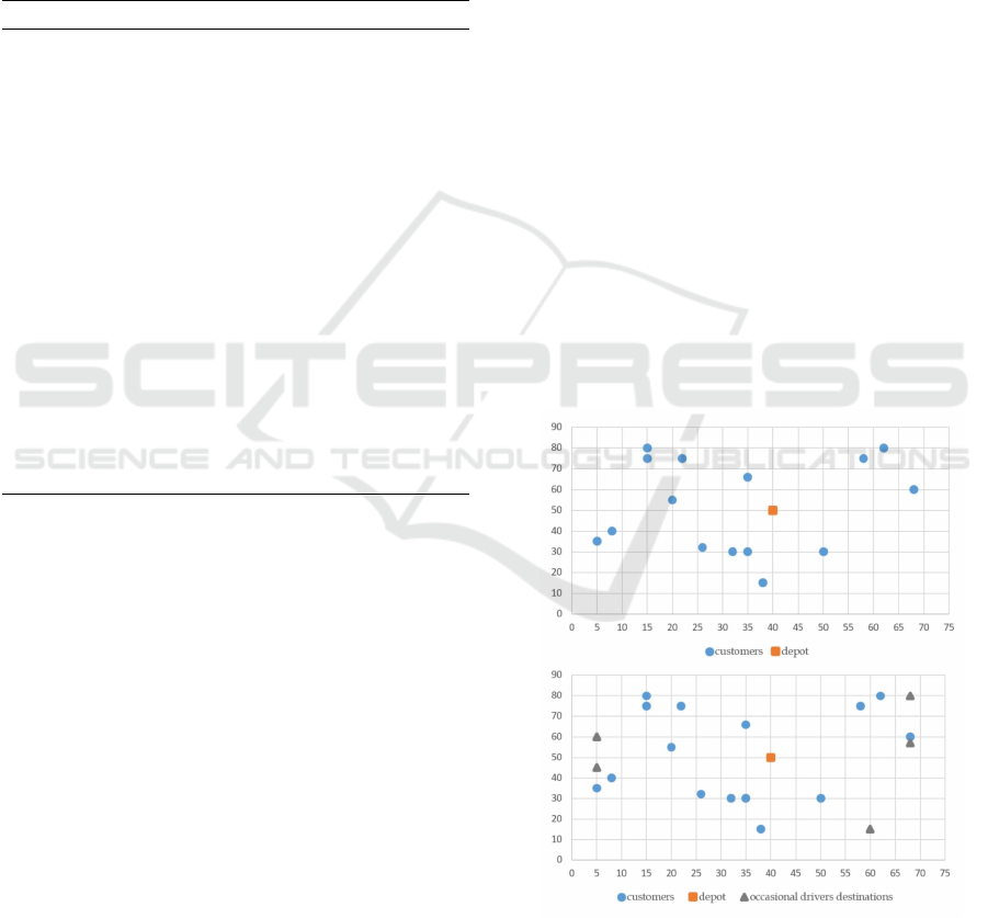
Figure 1 provides an example of an instance gen-

eration.

Figure 1: Generation of instance C103C15.

Table 2 reports the characteristics of the instances

in terms of number of customers |C|, number of clas-

sical vehicles P, number of available ODs |K|, capac-

ity of the vehicles Q, and capacity of the ODs Q

ICORES 2020 - 9th International Conference on Operations Research and Enterprise Systems

274

Table 2: Parameters setting for the generation of the in-

stances.

|C| P |K| Q Q

5 3 3 80 [10,25]

10 3 3 80 [10,30]

15 3 5 80 [15,35]

25 5 10 100 [20,40]

50 8 15 200 [20,40]

100 10 30 400 [20,40]

4.2 Evaluation of the VNS Perfomance

In order to assess the performance of our VNS, we

ﬁrst solved the problem to optimality with CPLEX,

we then compared the results with those obtained by

the VNS. We set k

max

= 50 and improve = 15.

Tables 3 to 5 compare the solutions obtained for

small-size instances. For each table and each algo-

rithm (VNS and resolution with CPLEX), the ﬁrst

column displays the name of the instance, the second

one the execution time [ms], the third one is the total

cost, the fourth and the ﬁfth columns show the number

of classical vehicles (CV) and OD vehicles used, re-

spectively. The two last columns display the optimal-

ity gap on cost, calculated as g

cost

= (Objective

VNS

−

Objective

CPLEX

)/Objective

CPLEX

and the Speedup

(Sp-up), calculated as the ratio between the execution

time of CPLEX and that of the heuristic, respectively.

The VNS looks very effective, indeed, it ﬁnds an op-

timal solution for the majority of instances. In par-

ticular, Table 3 and Table 4 highlight the efﬁciency

of the VNS for instances with ﬁve and 10 customers.

The proposed algorithm ﬁnds the optimal solution for

all instances. As shown in Table 5, the VNS is also

highly effective for instances with 15 customers, the

average gap is 0.3% and it ﬁnds the optimal solution

for 75% of the instances. Looking at column Sp-up in

Tables 3 to 5, it is worth observing that our approach

is also more efﬁcient than CPLEX. We can summarize

that the VNS ﬁnds the optimal solutions for the ma-

jority of the instances within short computing times.

Our approach clearly outperforms CPLEX.

Table 3: Results for ﬁve customers and three occasional

drivers instances.

VNS OPT

Test Time Cost CV OD Time Cost CV OD gap Sp-

C101C5 99.0 145.4 1 2 60.0 145.4 1 2 0.0% 0.6

C103C5 22.0 111.6 1 2 24.0 111.6 1 2 0.0% 1.1

C206C5 10.0 159.6 1 1 30.0 159.6 1 1 0.0% 3.0

C208C5 5.0 131.9 1 1 38.0 131.9 1 1 0.0% 7.6

R104C5 20.0 107.2 1 2 28.0 107.2 1 2 0.0% 1.4

R105C5 2.0 143.1 2 1 12.0 143.1 2 1 0.0% 6.0

R202C5 23.0 129.5 2 1 46.0 129.5 2 1 0.0% 2.0

R203C5 20.0 170.1 1 1 28.0 170.1 1 1 0.0% 1.4

RC105C5 20.0 143.1 1 2 16.0 143.1 1 2 0.0% 0.8

RC108C5 12.0 164.0 1 2 21.0 164.0 1 2 0.0% 1.8

RC204C5 5.0 107.0 1 2 30.0 107.0 1 2 0.0% 6.0

RC208C5 5.0 124.9 1 2 25.0 124.9 1 2 0.0% 5.0

Avg 20.3 136.5 1.2 1.6 29.8 136.5 1.2 1.6 0.0% 3.1

Table 4: Results for 10 customers and three occasional

drivers instances.

VNS OPT

Test Time Cost CV OD Time Cost CV OD gap Sp-

C101C10 1028.0 283.2 3 2 127 283.2 3 2 0.0% 0.1

C104C10 16.0 242.4 2 3 315 242.4 2 3 0.0% 19.7

C202C10 36.0 175.4 2 3 51 175.4 2 3 0.0% 1.4

C205C10 16.0 184.7 2 2 97 184.7 1 2 0.0% 6.1

R102C10 19.0 166.4 1 2 68 166.4 1 2 0.0% 3.6

R103C10 286.0 154.0 2 1 316 154.0 2 1 0.0% 1.1

R201C10 99.0 185.2 2 2 73 185.2 3 2 0.0% 0.7

R203C10 17.0 132.9 1 3 100 132.9 1 3 0.0% 5.9

RC102C10 46.0 331.8 2 2 78 331.8 2 2 0.0% 1.7

RC108C10 263.0 330.1 2 2 184 330.1 2 2 0.0% 0.7

RC201C10 28.0 231.1 2 2 34 231.1 2 2 0.0% 1.2

RC205C10 23.0 260.3 2 2 44 260.3 2 2 0.0% 1.9

Average 156.4 223.1 1.9 2.2 123.9 223.1 1.9 2.2 0.0% 3.7

Table 5: Results for 15 customers and ﬁve occasional

drivers instances.

VNS OPT

Test Time Cost CV OD Time Cost CV OD gap Sp-

C103C15 215.0 206.5 1 5 4092.0 206.5 1 5 0.0% 19.0

C106C15 99.0 161.9 2 5 718.0 161.9 2 5 0.0% 7.3

C202C15 85.0 338.3 2 4 2786.0 332.9 2 4 1.6% 32.8

C208C15 10.0 304.7 3 3 351.0 304.7 3 3 0.0% 35.1

R102C15 129.0 297.8 3 4 191.0 297.8 3 3 0.0% 1.5

R105C15 247.0 215.8 2 5 127.0 215.8 1 5 0.0% 0.5

R202C15 30.0 324.4 3 4 5515.0 324.4 3 4 0.0% 183.8

R209C15 782.0 239.4 3 3 3648.0 239.4 3 3 0.0% 4.7

RC103C15 51.0 341.6 3 3 2348.0 341.6 3 3 0.0% 46.0

RC108C15 72.0 252.6 2 5 13848.0 248.6 2 5 1.6% 192.3

RC202C15 144.0 357.3 3 4 390.0 356.3 3 5 0.3% 2.7

RC204C15 23.0 341.1 2 3 831837.0 341.1 2 3 0.0% 36166.8

Average 157.3 281.8 2.4 4.0 72154.3 280.9 2.3 4.0 0.3% 3057.7

4.3 Numerical Results on the

Medium-size and Large-size

Instances

We now present the computational results on in-

stances with 25, 50 and 100 customers.

with k

max

= 200 and improve = 150.

Tables 6 to 8 summarize the results obtained for

this set of instances. For each table, the ﬁrst column

displays the name of the instance, the second one the

computational time [ms], the third one the total cost,

the fourth and ﬁfth columns show the number of clas-

sical and OD routed vehicles, respectively. We also

report averages in the last line. Overall, the VNS ﬁnds

solutions within short computing times. Indeed, the

VNS solve instances with 25 nodes in about one sec-

ond, with 50 nodes in about four seconds, and with

100 nodes in about 20 seconds (about three time less

than the time spent by CPLEX to solve instances with

15 customers). Table 6 shows that the solutions gen-

erated use, on average, about six ODs out of 10 and

about four traditional vehicles. Tables 7 exhibits the

same trend. Indeed, the solutions use on average eight

out of 15 ODs. The use of ODs becomes more inter-

esting on instances with 100 nodes. Looking at Table

8, it is clear that the majority of the generated solu-

tions use a huge number of ODs.

The advantages of using ODs in transportation

A Variable Neighborhood Search for the Vehicle Routing Problem with Occasional Drivers and Time Windows

275

Table 6: Results for instances with 25 customers.

Test Time Cost # traditional # occasional

C101C25 1684.0 299.2 4 3

C102C25 2563 350.4 5 2

C103C25 2381.0 331.9 3 8

C104C25 716.0 326.8 4 3

C105C25 1028.0 350.8 5 1

R101C25 629.0 326.5 3 9

R102C25 1214.0 293.3 1 10

R103C25 828.0 297.5 2 8

R104C25 754.0 306.7 2 9

R105C25 149.0 288.3 2 9

RC101C25 4234.0 560.7 5 3

RC102C25 2387.0 539.1 5 3

RC103C25 772.0 455.9 4 7

RC104C25 1240.0 455.3 4 6

RC105C25 2058.0 538.1 5 3

Average 1509.1 381.4 3.6 5.6

Table 7: Results for instances with 50 customers.

Test Time Cost # traditional # occasional

C101C50 1348 521.1 4 7

C102C50 9452 443.4 3 12

C103C50 1355 447.9 3 9

C104C50 19422 437.2 4 7

C105C50 761 461.7 3 9

R101C50 830 727.3 5 15

R102C50 5283 707.4 4 14

R103C50 2801 539.4 3 9

R104C50 1045 509.6 3 11

R105C50 951 662.7 5 6

RC101C50 1247 516.8 3 12

RC102C50 5960 547.8 4 7

RC103C50 17246 561.6 4 7

RC104C50 8229 601.1 4 6

RC105C50 2370 660.9 6 3

Average 5220.0 556.4 3.9 8.9

Table 8: Results for instances with 100 customers.

Test Time Cost # traditional # occasional

C101 927.0 1344.5 5 28

C102 3031 1376.9 6 24

C103 1036.0 1230.5 6 27

C104 37963.0 1172.1 6 19

C105 1246.0 1431.6 6 27

R101 18538.0 1384.0 9 19

R102 34872.0 1292.9 8 11

R103 23756.0 1157.2 7 13

R104 86965.0 880.6 4 12

R105 6707.0 1337.4 8 11

RC101 23431.0 1425.3 8 27

RC102 25884.0 1488.5 8 9

RC103 30032.0 1165.5 7 10

RC104 11398.0 1085.5 6 17

RC105 769.0 1295.1 9 29

Average 20437.0 1271.2 6.9 18.9

planning have been deeply analyzed in (Macrina

et al., 2017), where the effectiveness of delivery con-

ﬁgurations that rely on the use of ODs is compared

with that obtained by using traditional vehicles only.

It has been shown that the use of the ODs may im-

prove the routing plans, generating an interesting cost

saving of about 12.5% on small-size instances. On

the other hand, general-purpose optimization solvers,

like CPLEX, are not able to solve instances with more

than 15 customers and ﬁve ODs. Thus, it is evident

that the availability of a heuristic approach allows to

fully exploit the beneﬁts of crowd-shipping also in

case of large-size instances. Our computational study

conﬁrms that the number of ODs used increases with

the increase of the size of the instances. From a prac-

tical point of view, this not only means that a cost

improvement for the transportation companies is ob-

tained, but also a reduction of the delivery times is

determined, with a consequent improvement of the

quality of service offered to customers.

5 CONCLUSIONS

We have proposed a variable neighborhood search

heuristic for the vehicle routing problem with occa-

sional drivers, time windows, and multiple deliveries.

In order to assess the performance of our proposed

heuristic, we have solved the problem with CPLEX

for small-size instances. We have then conducted a

comparative analysis. We have shown that our heuris-

tic is highly performing in terms of effectiveness and

efﬁciency. Overall, the heuristic is less time consum-

ing than CPLEX. We have also shown that it can solve

large-size instances within a limited computing time.

ACKNOWLEDGEMENTS

This work was partly supported by MIUR

“PRIN2015” funds, project: “Transportation

and Logistics in the Era of Big Open Data” -

2015JJLC3E 003 - CUP H52F15000190001.

REFERENCES

Archetti, C., Savelsbergh, M. W. P., and Speranza, M. G.

(2016). The vehicle routing problem with occasional

drivers. European Journal of Operational Research,

254:471–480.

Arslan, A. M., Agatz, N., Kroon, L., and Zuidwijk, R.

(2016). Crowdsourced delivery: A dynamic pickup

and delivery problem with ad-hoc drivers. Technical

report, ERIM, Report Series Reference.

Barr, A. and Wohl, J. (2013). Exclusive: Wal-Mart may

get customers to deliver packages to online buyers.

REUTERS - Business.

Bensinger, G. (2015). Amazon’s next delivery drone: You.

Wall Street Journal.

Dahle, L., Andersson, H., and Christiansen, M. (2017).

The vehicle routing problem with dynamic occasional

drivers. In Bektas¸, T., Coniglio, S., Martinez-Sykora,

A., and Voß, S., editors, Computational Logistics,

pages 49–63, Cham. Springer International Publish-

ing.

Dahle, L., Andersson, H., Christiansen, M., and Speranza,

M. G. (2019). The pickup and delivery problem with

time windows and occasional drivers. Computers and

Operations Research, 109:122–133.

Dayarian, I. and Savelsbergh, M. (2017). Crowdshipping

and same-day delivery: employing in-store customers

ICORES 2020 - 9th International Conference on Operations Research and Enterprise Systems

276

to deliver online rders. Technical report, optimization-

online.

eMarketer (2018). Retail ecommerce sales worldwide,

2017–2021. https://www.emarketer.com/chart/

219928/retail-ecommerce-sales-worldwide-2017-

2021-trillions-change-of-total-retail-sales.

Gdowska, K., Viana, A., and Pedroso, J. P. (2018). Stochas-

tic last-mile delivery with crowdshipping. Transporta-

tion Research Procedia, 30:90 – 100.

Landa, R. (2015). Thinking Creatively in the Digital Age.

Nimble, Blue Ash, Ohio, 1

edition.

Macrina, G., Di Puglia Pugliese, L., Guerriero, F., and La-

gan

a, D. (2017). The vehicle routing problem with

occasional drivers and time windows. In Sforza, A.

and Sterle, C., editors, Optimization and Decision Sci-

ence: Methodologies and Appliations, volume 217

of Springer Proceedings in Mathematics & Statistics,

pages 577–587, Cham, Switzerland. ODS, Sorrento,

Italy, Springer.

Macrina, G., Di Puglia Pugliese, L., Guerriero, F., and La-

porte, G. (2020). Crowd-shipping with time windows

and transshipment nodes. Computers and Operations

Research, 113.

Macrina, G. and Guerriero, F. (2018). The green vehicle

routing problem with occasional drivers. In Daniele,

P. and Scrimali, L., editors, New Trends in Emerging

Complex Real Life Problems. Springer International

Publishing, Springer New York LLC.

Solomon, M. M. (1987). Algorithms for the vehicle rout-

ing and scheduling problems with time window con-

straints. Operations Research, 35:254–265.

A Variable Neighborhood Search for the Vehicle Routing Problem with Occasional Drivers and Time Windows

277