Scene Adaptive Structured Light 3D Imaging

Tomislav Pribanic

, Tomislav Petkovic

, David Bojanic

, Kristijan Bartol

and Mohit Gupta

Faculty of Electrical Engineering and Computing, University of

Zagreb, Unska 3, Zagreb, Croatia

Department of Computer Science, University of Wisconsin, Madison, WI, U.S.A.

Keywords: 3D Imaging, Structured Light, Time-of-Flight, Depth Precision.

Abstract: A 3D structured light (SL) system is one powerful 3D imaging alternative which in the simplest case is

composed of a single camera and a single projector. The performance of 3D SL system has been studied

considering many aspects, for example, accuracy and precision, robustness to various imaging factors,

applicability to a dynamic scene capture, hardware and image processing complexity, to name but a few. In

this work we consider the spatial projector-camera set up and its influence on the uncertainty of points’ depth

reconstruction. In particular, we show how a depth precision is in a great extent determined by the angle of

pattern projection and the angle of imaging from a projector and a camera, respectively. For a fixed camera

projector configuration, those angles are scene dependent for various points in space. Consequently, the

attainable depth precision will typically vary considerably across the volume of reconstruction which is not a

desirable property. To that end, we study a scene dependent 3D imaging approach during which we propose

how to conveniently detect points with a lower depth precision and to influence other factors of a depth

precision, in order to improve a depth precision in scene parts where necessary.

1 INTRODUCTION

The study on 3D imaging system design has attracted

a great deal of attention in computer vision. There has

been many methods and systems proposed (Chen,

Brown, & Song, 2000). A particularly interesting

ones are active illumination 3D imaging systems

where, besides a camera, an active source of

illumination is introduced. The most representative

ones are photometric systems (Barsky & Maria,

2003), time-of-flight (ToF) cameras (Hansard, Lee,

Choi, & Horaud, 2012) and structured light (SL)

systems (Geng, 2011). SL has proven to be one of the

most accurate and robust methods proposed and

analyzed (Salvi, Fernandez, Pribanic, & Xavier,

2010). In SL an illumination source is typically a

projector. The main task of a projector is to project

pattern(s) in the scene. That is especially beneficial

when a natural scene has a low texture since SL is

triangulation-based 3D imaging system and, in order

to triangulate 3D point position, it is necessary to find

https://orcid.org/0000-0002-5415-3630

https://orcid.org/0000-0002-3054-002X

https://orcid.org/0000-0002-2400-0625

https://orcid.org/0000-0003-2806-5140

the correspondent projector and camera image

coordinates. Having basically two different pieces of

hardware HW, i.e. a camera and a projector, opened

an additional vast amount of research possibilities to

study the performance of SL systems. Naturally, the

reconstruction accuracy and precision aspects have

been given perhaps the most attention. To that end,

different factors and system design issues have been

analyzed and various measures have been proposed in

order to improve the accuracy and precision.

However, somewhat surprisingly and to the best of

our knowledge, there is relatively less work about the

spatial geometrical set up between a camera and a

projector (Liu & Li, 2014). We note that besides a

camera projector baseline, two other most obvious

factors defining a geometry of 3D reconstruction are

the angle of projector’s pattern projection and the

angle of camera imaging (angles α and β in Figure 1).

In this work our main contributions are related to

those two angles and to their influence on the depth

precision. First, we derive an expression clearly

576

Pribanic, T., Petkovic, T., Bojanic, D., Bartol, K. and Gupta, M.

Scene Adaptive Structured Light 3D Imaging.

DOI: 10.5220/0009189905760582

In Proceedings of the 15th International Joint Conference on Computer Vision, Imaging and Computer Graphics Theory and Applications (VISIGRAPP 2020) - Volume 4: VISAPP, pages

576-582

ISBN: 978-989-758-402-2; ISSN: 2184-4321

showing the various factors determining the depth

precision of a SL system, two of which are the afore

mentioned angles of pattern projection and imaging.

We further demonstrate how those two angles change

across the scene, thus having a significant impact on

the expected depth precision throughout the scene.

Obviously, the pair of such angles are scene

dependent and for a general scene cannot be

anticipated in advance. we also provide a simple

measure on improving the depth precision for those

points in space where the particular angles cause an

unsatisfactory depth precision. In turn, the proposed

strategy allows scene dependent 3D imaging.

The remainder of this work is structured as

follows. We next briefly cover the related work on 3D

active imaging. Afterwards we derive an expression

for SL system depth precision, followed by the

experimental simulations of depth precision

dependency on angles of pattern projection and

imaging. In the same section we discuss possible

measures of improving the depth precision. At the end

we reflect on the possible future work and draw the

main paper conclusions.

2 RELATED WORK

A common approach to classify 3D imaging systems

is to divide them in the following three groups:

triangulation, interferometry and time-of flight

(Büttgen, Oggier, Lehmann, Kaufmann, &

Lustenberger, 2015). An even simpler classification

would be only in two groups: passive and active 3D

imaging systems. Within the active ones two most

notable representatives, and closely related to this

work, are structured light systems and time of flight

cameras which will be, therefore, in brief jointly

overviewed.

Due to a fact that an active source of illumination

has been utilized, a significant deal of work was

devoted to the performance error analyses where

multiple illuminations sources (3D imaging systems)

are simultaneously used. To prevent either interfering

one SL projector with another or one ToF LED (laser)

source with another several approaches have been

proposed: space division-multiple access (Jia, Wang,

Zhou, & Meng, 2016), wavelength-division multiple

access (Bernhard & Peter, 2008), time-division

multiple access, frequency-division multiple access )

(Petković, Pribanić, & Đonlić, 2017), and finally, in

the case of ToFs, a code-division multiple access

(Whyte, Payne, Dorrington, & Cree, 2010).

When analyzing the performance of a single 3D

imaging system, a significant work was done, mostly

in the field of ToFs, studying hardware itself w.r.t. to

various factors such as power budget, quantum noise

and thermal noise (Lange & Seitz, 2001); or

integration time related error and built-in pixel related

error (Foix, Alenya, & Torras, 2011). On the other

hand, SL system performance has been analyzed

mainly in the hardware agnostic manner, i.e. more in

the image processing sense by trying to identify

potential errors during pattern(s) (de)coding process

(Horn & Kiryati, 1997) and/or by finding the optimal

coding scheme (Gupta & Nakhate, A Geometric

Perspective on Structured Light Coding, 2018). That

is in a way understandable since in terms of signal

processing ToF is generally based on two or three

principles: continuous/discrete and direct time of

flight (Horaud, Hansard, Evangelidis, & Ménier,

2016). On the other hand, SL has richer alternatives

regarding the various types of patterns to be projected

and subsequently processed, particularly using color

patterns for dynamic scenarios (Petković, Pribanić, &

Đonlić, 2016). In that sense a high emphasis was put

on a design of patterns to be projected (Mirdehghan,

Chen, & Kutulakos, 2018). Interestingly, certain

hardware design proposed solutions for ToF, e.g.

epipolar time of flight imaging (Achar, Bartels,

Whittaker, Kutulakos, & Narasimhan, 2017), are

applicable for SL too.

One of the main differences between ToF and SL

is the former does not have the baseline involved

since ToF illumination source and camera are

generally assumed to be collocated. In terms of the

baseline, an interesting work has been done in SL

when the baseline is very small which simplifies the

process of finding a projected code in cameras images

(Saragadam, Wang, Gupta, & Nayar, 2019).

Moreover, a close work to ours is the one analyzing

the influence of the short projector-camera baseline

on the performance (Liu & Li, 2014). Similarly

(Bouquet, Thorstensen, Bakke, & Risholm, 2017)

compares the performance 3D SL and ToF systems,

but without any relation to the geometrical

configuration between the camera and the projector.

To the best of our knowledge none of the mentioned

works are specially concentrated on the analyses of

the pattern projection angle and the camera imaging

angle and their impact on the estimated depth

precision.

Scene Adaptive Structured Light 3D Imaging

577

3 DEPTH PRECISION OF SL 3D IMAGING SYSTEM

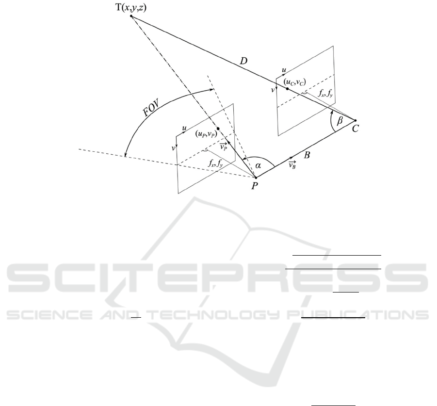
Figure 1 A: 3D point T, at the depth D from the camera (C), is projected in the camera (C) image at (u

, v

) and in the projector

(P) image at (u

, v

). Backprojected rays to the point T from the projector and the camera form with the baseline B the angles

α and β, respectively. FOV stands for a projector’s field of view. f

and f

are the effective focal lengths in the horizontal and

vertical direction, receptively.

We start by introducing the basic principle behind

phase shifting (PS) method which is very likely the

most notable SL pattern strategy (Salvi, Fernandez,

Pribanic, & Xavier, 2010). PS consists of sequentially

projecting a number (N≥3) of periodic sine patterns,

shifted by some phase shift 𝜑



∙



∙𝑖, where i=0, 1,

… N-1. The projected patterns are imaged by a

camera and then processed to compute a wrapped

phase φ, based on which the correspondence between

projector and camera image pixels can be established.

The intensity I

observed at some camera pixel can be

modeled as follows:

𝐼



𝐴

∙sin

(

𝜑+𝜑



)

+𝐶

(1)

where A is the brightness when projector projects its

full intensity (A is related to 3D points reflectivity and

propagation loss), φ is the unknown phase, φ

is the

known relative phase shift at which a particular pattern

was projected, and C represents the contribution from

a background illumination. Evidently having three

unknowns (A, φ and C) there are at least N=3 shifts

(projected patterns) needed to recover all three

unknowns. In practice to cope with the noise at least

four shifts are normally used, both in SL and ToF

systems also (Büttgen, Oggier, Lehmann, Kaufmann,

& Lustenberger, 2015), which allows to recover the

unknowns:

𝐴



(𝐼



−𝐼



)



+(𝐼



−𝐼



)



𝜑=tan





𝐼



−𝐼



𝐼



−𝐼





𝐶=

𝐼



+𝐼



+𝐼



+𝐼



(2)

We next derive a depth precision of the SL

system. Figure shows rectified, but still a very

general relationship between a projector, a camera

and some triangulated point in space. Using the law

of sines, we derive an expression for the depth D:

𝐷=

𝐵∙sin

(

𝛼

)

sin

(

𝛼+𝛽

)

(3)

where B is projector-camera baseline, and given some

point T, α is projector pattern projection angle with

the respect to baseline B and β is a camera imaging

angle with the respect to baseline B too. Depth

precision can be quantitively estimated as a depth

uncertainty where the cause of uncertainty can be

attributed to the noise in measurements I

of Eq. (1).

In particular, a standard deviation σ

of depth is

commonly estimated using the expression for the

error propagation:

VISAPP 2020 - 15th International Conference on Computer Vision Theory and Applications

578

𝜎







𝜕𝐷

𝜕𝐼







∙𝑉𝑎𝑟

(

𝐼



)



𝑖=0

(4)

where the variance Var(I

) is modeled as being equal

to the signal level (Lange & Seitz, 2001). According

to the expression (3), the depth D is explicitly

dependent on the angles α and β. However, angle α

can be expressed as a function of the phase φ (2)

which in turn provides a relationship to the

measurements I

. Hence, using the chain rule the

partial derivative







can be expressed as:

𝜕𝐷

𝜕𝐼



𝜕𝐷

𝜕𝛼

𝜕𝜑

𝜕𝐼



(5)

Based on Eq. (3), the first factor in Eq. (5) is readily

computed:

𝜕𝐷

𝜕𝛼

𝐵·sin𝛽

𝑠𝑖𝑛



(

𝛼+𝛽

)

(6)

The actual relationship between the angle α and the

phase φ is less obvious. According to Figure 1, the

vector v

pointing back in space in the direction of the

spatial point T can be computed based on the

projector calibration matrix K

and on the projector

image point p=[u

𝐾



=

𝑓



0𝑢



𝑓



𝑣



001



𝑣



=𝐾





∙𝑝=

⎣

⎢

⎡

𝑢



−𝑢



𝑓



𝑣



−𝑣



𝑓



⎦

⎥

⎤



(7)

where (u

, v

) are projector image coordinates,

, v

) is the position of the principal point in the

projector image. f

and f

are effective focal lengths

in horizontal and vertical direction, respectively. For

the simplicity of exposition and without loss of

generality we can set an image component coordinate

u as being identical to the wrapped phase φ. Next, the

angle α is immediately determined by a dot product

between the vector v

and the baseline B direction

vector v

, where v

can be taken as a unit vector.

cos𝛼=

𝑑𝑜𝑡(𝑣



,𝑣



)

𝑣



∙

𝑣



𝑑𝑜𝑡(𝑣



,𝑣



)

𝑣



(8)

Evidently this poses a nonlinear relationship between

the angle α and the wrapped phase φ. Fortunately, the

angle α typically spans values where the cos𝛼 𝑖𝑠

fairly linear w.r.t. its argument (unless a wide-angle

optics for a projector is used). Therefore, similarly as

in (Bouquet, Thorstensen, Bakke, & Risholm, 2017),

we approximate the relationship between the angle α

and the wrapped phase φ with a linear function. Using

fairly straightforward geometry relations, depicted on

Figure , it can be shown that:

𝛼≈-FOV/φ_MAX ∙𝜑+





(9)

where FOV is projector’s field of view. Eq. (9) finally

determines the partial derivative





=−







and

simplifies the original (4) to.

𝜎



𝐵·sin𝛽∙𝐹𝑂𝑉

sin



(

𝛼+𝛽

)

∙𝜑



∙





𝜕𝜑

𝜕𝐼







∙𝐼





𝑖=0

(10)

The sum of partial derivatives under the square root

from (10), using the relations (1) and (2), will yield

√



√∙

and will ultimately define the final expression for

the depth standard deviation σ

𝜎



𝐷



·𝐹𝑂𝑉∙

√

𝐶

𝐵∙𝜑



∙√2∙𝐴

∙

sin𝛽

𝑠𝑖𝑛



𝛼

𝜎



𝐵·𝐹𝑂𝑉∙

√

𝐶

𝜑



∙

√

2∙

𝐴

∙

sin𝛽

𝑠𝑖𝑛



(

𝛼+𝛽

)

(11)

Here we point out the dependence of σ

on the part

we call the angle factor 𝐴𝐹=







(



)

. In the next

section we show how AF affects the amount of

standard deviation σ

across the reconstruction whole

volume.

4 RESULTS AND DISCUSSION

In this section we first show how the angle factor AF

varies across a 3D imaging scene. Then we use Monte

Carlo approach in the synthetic experiments to

estimate the depth standard variation σ

for various

points in the 3D space. Finally we propose and

discuss strategies to improve depth precision for the

desired portion of space, in order to achieve a more

uniform depth precision values across the volume. To

that end, and without loss of generality, we assume

one plausible projector-camera set up where projector

and camera images are epipolary rectified (Fusiello,

Trucco, & Verri, 2000) and with the following

parameters: the baseline B=300mm, the effective

focal lengths in pixels f

=fy=1000, image resolution

Scene Adaptive Structured Light 3D Imaging

579

(u, v)=(1024, 768), the principal point coordinates

, v

)=(512, 384).

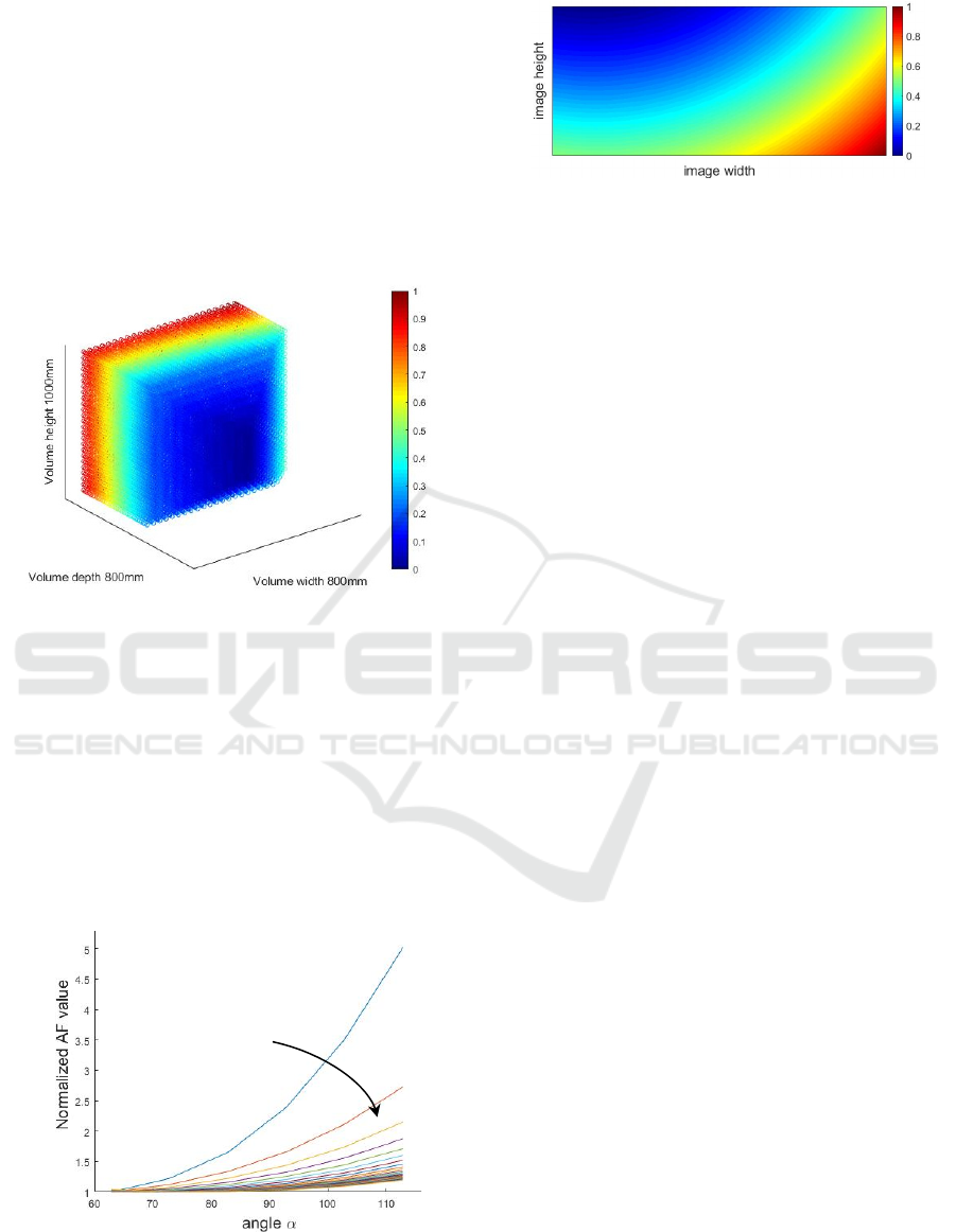
Figure 2 visualizes the change of AF for a given

volume and at the standoff distance 400mm from the

3D SL scanner. In the case of this rectified projector-

camera set up, AF factor increases (a depth precision

becomes worse) almost linearly along the volume

depth. However, besides volume depth alone, which

can be fairly arbitrary defined, we are even more

interested about AF dependency of the depth D wrt to

the camera itself.

Figure 2: The relative change of AF across the 3D imaging

volume 800mm×800mm×1000mm(width×depth×height).

3D scanner standoff distance is 400mm.

Figure 3 shows, for a sequence of constant depths

D, how AF changes as the angle α changes, spanning

the entire projector’s FOV angle. Given the current

projector-camera arrangement it turns out that at

some constant depth D, AFs become worse and worse

as the angle α increases. In fact, the relative

discrepancy between points having a small AF and

points having a big AF is more evident as the depth D

is smaller.

Figure 3: Each solid curve corresponds to a constant depth.

Going from the top curve to the bottom, depth D changes

from 350mm to 1000mm. Values within each curve are

normalized on the smallest AF value for that curve (depth).

Figure 4: A camera image of the 3D plane of points, parallel

to the projector-camera image plane, where the intensity

represents the values of AF.

Figure 4 presents another alternative overlook on

the issue. In this case points in 3D plane, at the

standoff distance of about 300mm and parallel to the

projector-camera image planes, are projected to the

camera image where for each point the value AF is

shown as the intensity. Going from the upper left

corner to the lower right corner, a diversity of AF

values is witnessed, even though the points are in the

plane parallel to the projector/camera images. Thus,

one must not conclude, as may seem at the first glance

based solely on the previous Figure 2, that in planes

parallel to the projector-camera image plane there are

no notable changes in the AF values. Therefore, in the

case of a general scene it is reasonable to expect

points having different values for the angles α and β

not only at different depths D, but also within the

same depth D as well. In turn, a diverse set of AF

values is expected to be present. The fact is that

having point clouds reconstructed with the

significantly different precision values per individual

points may impair further processing on the point

cloud itself.

The natural question raises on how to improve the

depth precision for a desired portion of 3D points or

even for individual points. Examining the expression

(11) we notice the depth standard variation σ

controlled by several parameters. The one most

convenient to control is likely to be the value A

dictated by the strength of the illumination source.

Using the illumination source with an adjustable

illumination power over different portion of projector

images/patterns, such as in (Gupta, Yin, & Nayar,

Structured Light In Sunlight, 2013), it is possible to

relatively easily decrease or increase the value of A

during the scanning (pattern projection). In turn this

assures a seamless approach to directly impact the

depth standard variation σ

in the areas where needed.

Our proposed approach initially scans 3D scene

simply to get an estimate on AF values. This intial

scan is done in practice using the fewest number of

patterns possible since we just need a rough estimate

of AF values which does not require highly accurate

and precise 3D reconstruction. Afterward, the scene

th D increases

VISAPP 2020 - 15th International Conference on Computer Vision Theory and Applications

580

is re-scanned using the full set of patterns and with

the appropriate strengths of the illuminations across

the scene.

In attempt to verify the crucial part of our

approach we perform the following simulation. We

randomly sample M=100 points from the volume as

defined in Figure 2. Such point set will exhibit a

significantly different AF values. For each of these

3D points we estimate the depth standard variation σ

using the Monte Carlo simulation. That is, we assume

an additive Gaussian noise on the image values I

from Eq.(1), with noise variance equal to I

, and

generate such random noise values in order to

compute the phase φ from Eq.( 2). Knowing φ we can

eventually estimate noisy depth D. Repeating the

experiment a number of times (N=10000) for each

known 3D point, allows us to estimate directly the

depth standard deviation σ

. According to our theory

we expect to see a proportional relation between the

estimated depth standard deviation and the

corresponding AF of a certain point. In another

words, the ratios between the different depth standard

deviations σ

should be the same as the ratios of AF’s.

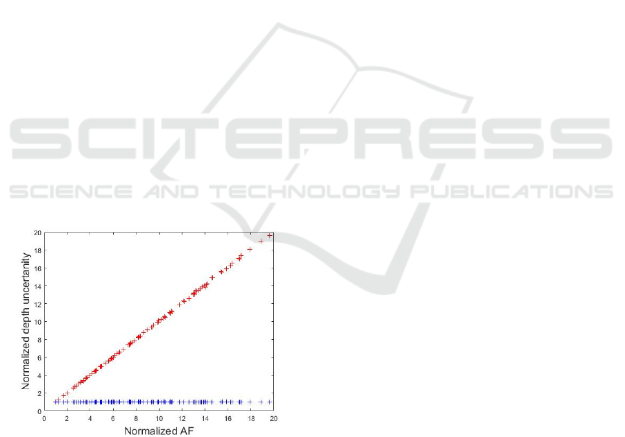
Following the above-mentioned simulation, Figure 5

presents on the vertical axis the estimated depth

standard deviations normalized to the smallest one in

the randomly chosen set of the above mentioned

M=100 points. On the horizontal axis the

corresponding AF’s are normalized to the AF of the

smallest estimated depth standard deviation. In Figure

5 emerges (almost) a straight diagonal (red) line

which confirms our predicted theory.

Figure 5: Diagonal (red) line: Verification of the

relationship between the depth precision and AF.

Horizontal (blue) line: After the proposed adjustment of

illuminations source strength, depth precision becomes

invariant w.r.t. AF.

Next, we look for the ratio of AF’s with the

respect to the point having the smallest (within

randomly chosen set of M=100 points) estimated

depth standard deviation and we aim to appropriately

increase the illuminations strength of all other points

in order to achieve the same depth precision. Thus,

we run another Monte Carlo simulation for estimation

of standard deviations, but this time with the suitably

increased value A for each of the remaining points.

Figure 5 shows a straight horizontal (blue) line

proving that after the proposed adjustment of the

illumination strength a depth precision (an estimated

depth standard variation) is uniform across all 3D

points, i.e. it is independent of the AF.

5 CONCLUSIONS

In this work we have proposed a method for scene

dependent 3D imaging aimed at improving the depth

precision at various 3D points in space. We have

begun by developing a theoretical framework

explaining the depth precision in 3D imaging system

based on the SL principle. Within this framework we

have identified several key factors determining a

depth precision, among which are the projector’s

angle of pattern projection and the camera’s angle of

imaging. We have proposed to analyze jointly the

influence of these two angles through a proposed

angle factor AF. Having established a clear

dependence of AF on the depth precision, we have

further proposed a simple approach to improve the

depth precision on the desired set of points, by

manipulating the strength of the illumination source.

The foreseen future work will include the

implementation and evaluation using the actual

hardware. In addition, we plan to consider the

improvement of depth precision using other factors

such as the number of phase shifts undertaken during

the phase shifting procedure.

ACKNOWLEDGEMENTS

This work has been supported in part by Croatian

Science Foundation under the project IP-2018-01-

8118, in part by the European Regional Development

Fund under the grant KK.01.1.1.01.0009

(DATACROSS) and in part by the Fulbright U.S.

Visiting Scholar Program.

Scene Adaptive Structured Light 3D Imaging

581

REFERENCES

Achar, S., Bartels, J. R., Whittaker, W. L., Kutulakos, K.

N., & Narasimhan, S. G. (2017). Epipolar time-of-flight

imaging. ACM Transactions on Graphics (TOG), 36(4),

371:1-37:8. doi:10.1145/3072959.3073686

Barsky, S., & Maria, P. (2003). The 4-Source Photometric

Stereo Technique for Three-Dimensional Surfaces in

the Presence of Highlights and Shadows. IEEE

Transactions on Pattern Analysis and Machine

Intelligence, 25(10), 1239-1252.

Bernhard, B., & Peter, S. (2008). Robust Optical Time-of-

Flight Range Imaging Based on Smart Pixel Structures.

IEEE Transactions on Circuits and Systems I, 55(6),

1512 - 1525.

Bouquet, G., Thorstensen, J., Bakke, K. A., & Risholm, P.

(2017). Design tool for TOF and SL based 3D cameras.

Optics Express, 25(22), 27758-27769. doi:10.1364/

OE.25.027758

Büttgen, B., Oggier, T., Lehmann, M., Kaufmann, R., &

Lustenberger, F. (2015). CCD/CMOS lock-in pixel for

range imaging: Challenges, Limitations and State-of-

the-Art. In In Proceedings of 1st Range Imaging

Research Day (pp. 21-32).

Chen, F., Brown, G., & Song, M. (2000). Overview of

three-dimensional shape measure- ment using optical

methods. Optical Engineering, 31(1), 10-22.

Foix, S., Alenya, G., & Torras, C. (2011). Lock-in Time-of-

Flight (ToF) Cameras: A Survey. 11(3), IEEE Sensors

Journal. doi:10.1109/JSEN.2010.2101060

Fusiello, A., Trucco, E., & Verri, A. (2000). A Compact

Algorithm for Rectification of Stereo Pairs. Machine

Vision and Applications, 12(1), 16-12. doi:doi.org/

10.1007/s001380050

Geng, J. (2011). Structured-light 3D surface imaging: a

tutorial. Advances in Optics and Photonics, 3(2), 128-

160. doi:doi.org/10.1364/AOP.3.000128

Gupta, M., & Nakhate, N. (2018). A Geometric Perspective

on Structured Light Coding. European Conference on

Computer Vision (pp. 90-107). Munich: Springer,

Cham. doi:10.1007/978-3-030-01270-0_6

Gupta, M., Yin, Q., & Nayar, S. K. (2013). Structured Light

In Sunlight. IEEE International Conference on

Computer Vision (ICCV), (pp. 1-8). Sydney.

Hansard, M., Lee, S. L., Choi, O. C., & Horaud, R. (2012).

Time of Flight Cameras: Principles, Methods, and

Applications. London: Springer. doi:10.1007/978-1-

4471-4658-2

Horaud, R., Hansard, M., Evangelidis, G., & Ménier, C.

(2016). An Overview of Depth Cameras and Range

Scanners Based on Time-of-Flight Technologies. (S.

Verlag, Ed.) Machine Vision and Applications, 27(7),

1005-1020. doi:10.1007/s00138-016-0784-4

Horn, E., & Kiryati, N. (1997). Toward optimal structured

light patterns. Proceedings. International Conference

on Recent Advances in 3-D Digital Imaging and

Modeling (pp. 28-35). Ottawa: IEEE. doi:10.1109/

IM.1997.603845

Jia, T., Wang, B., Zhou, Z., & Meng, H. (2016). Scene

depth perception based on omnidirectional structured

light. IEEE Transactions on Image Processing, 25(9),

4369 - 4378. doi:10.1109/TIP.2016.2590304

Lange, R., & Seitz, P. (2001). Solid-State Time-of-Flight

Range Camera. IEEE Journal of Quantum Electronics,

37(3), 390-397. doi:10.1109/3.910448

Liu, J., & Li, Y. (2014). Performance analysis of 3-D shape

measurement algorithm with a short baseline projector-

camera system. Robotics and Biomimetics, 1-10.

doi:doi.org/10.1186/s40638-014-0001-8

Mirdehghan, P., Chen, W., & Kutulakos, K. N. (2018).

Optimal Structured Light a la Carte. Computer Vision

and Pattern Recognition (CVPR, (pp. 6248-6257). Salt

Lake City. doi:10.1109/CVPR.2018.00654

Petković, T., Pribanić, T., & Đonlić, M. (2016). Single-Shot

Dense 3D Reconstruction Using Self-Equalizing De

Bruijn Sequence. IEEE Transactions on Image

Processing, 25(11), 5131-5144. doi:10.1109/TIP.2016.

2603231

Petković, T., Pribanić, T., & Đonlić, M. (2017). Efficient

Separation between Projected Patterns for Multiple

Projector 3D People Scanning. International

Conference on Computer Vision (ICCV): Workshop on

Capturing and Modeling Human Bodies, Faces and

Hands., (pp. 815-823). Venice.

Salvi, J., Fernandez, S., Pribanic, T., & Xavier, L. (2010).

A state of the art in structured light patterns for surface

profilometry. Pattern Recognition, 43(8), 2666-2680.

doi:doi.org/10.1016/j.patcog.2010.03.004

Saragadam, V., Wang, J., Gupta, M., & Nayar, S. (2019).

Micro-Baseline Structured Light. International

Conference on Computer Vision (ICCV), (str. 4049-

4058). Seoul.

Whyte, R. Z., Payne, A. D., Dorrington, A. A., & Cree, M.

J. (2010). Multiple range imaging camera operation

with minimal performance impact. IS&T/SPIE

Electronic Imaging, 7538, pp. 75380I-1-10. San Jose.

doi:10.1117/12.838271

VISAPP 2020 - 15th International Conference on Computer Vision Theory and Applications

582