
Possibilities of Predicting Arterial Pressure by Means of Heart Rate
Variability
Anton Yu Dolganov
a
Ural Federal University Yekaterinburg, Russian Federation
Keywords: Arterial Pressure, Heart Rate Variability, Machine Learning, Genetic Programming, Regression.
Abstract: The paper shows results of the study which aims to predict values of arterial pressure by means of heart rate
variability features. A total list of 64 features was tested, which included features in time and frequency
domain, as well as non-linear features. As a means of feature selection, the genetic programming was used.
In particular binary encoding was used for generation of features in combinations as well as degree of the
polynomial. Data of 50 students-volunteers recorded in sitting position was used. Results of the study suggests
that certain heart rate variability features can be used for prediction of the change of arterial pressure.
Perspectives and future plans for results improvement were described.
1 INTRODUCTION
Arterial hypertension is one of the most common
diseases of the cardiovascular system worldwide.
Sharp fluctuations in blood pressure can lead to a
deterioration in the patient's condition. It is especially
worth noting that the rate of change of pressure has a
great influence. Therefore, the task of continuous
monitoring of blood pressure becomes extremely
important and in demand (WHO, 2018).
Currently used long-term monitoring systems are
usually invasive (and can only be carried out under
clinical conditions), or intrusive (and do not allow
continuous measurements due to the influence of
residual occlusion). Therefore, methods of indirect,
non-invasive and non-intrusive assessment of blood
pressure are becoming more common.
Blood pressure depends on several factors, heart
rate is one of them. However, many other variables
also affect blood pressure, such as arterial stiffness,
blood viscosity, volume of blood pumped into the
aorta, microcirculation impedance, etc. Artificial
intelligence methods based on using the capabilities
of machine learning can help solve this problem. Such
an approach allows not only to formalize the
description of complex living systems and conduct
prognostic analysis, but also to find implicit patterns
in the data.
a
https://orcid.org/0000-0003-2318-9144
Most of the work in this area comes down to using
plethysmogram signals or a combination of
plethysmograms with an electrocardiogram, where
standard parameters are calculated, such as the arrival
time of the pulse, the period of the pulse ejection, the
pulse propagation time, and the pulse wave velocity
(Anisimov et al., 2014; Kurylyak et al., 2013;
Sannino et al., 2015). However, approaches that
combine several signals are not practical for everyday
use.
At the same time, the possibilities of using only
electrocardiogram signals in the task of indirectly
assessing blood pressure have not been sufficiently
studied. Available works, as a rule, are limited to a
rough prediction of the level of pressure (high, normal
or low) and do not allow to obtain accurate estimates
(Simjanoska et al., 2018, 2019).
In previous works, a study was carried out of the
found complexes of significant parameters of heart
rate variability to assess the effectiveness of
treatment, which showed the consistency of the
calculated estimates with blood pressure
measurements (Vladimir Kublanov & Dolganov,
2019). This indicates the prospects of using the
parameters of heart rate variability signals in the task
of indirect estimation of blood pressure.
348
Dolganov, A.
Possibilities of Predicting Arterial Pressure by Means of Heart Rate Variability.
DOI: 10.5220/0009183203480354
In Proceedings of the 13th International Joint Conference on Biomedical Engineering Systems and Technologies (BIOSTEC 2020) - Volume 4: BIOSIGNALS, pages 348-354
ISBN: 978-989-758-398-8; ISSN: 2184-4305
Copyright
c
2022 by SCITEPRESS – Science and Technology Publications, Lda. All rights reserved

2 MATERIALS AND METHODS
2.1 Biomedical Signals Data
Pilot study was performed in Research Medical and
Biological Engineering Centre of High Technologies
(Ural Federal University, Russian Federation). A total
of 50 students volunteers have performed in the study.
Prior to the biomedical signals acquisition the
participants were informed of the study paradigm and
gave the consent to participate in the study.
The diagram of the study is presented on Figure 1.
Figure 1: Study Timeline.
All subjects were sitting during the whole Study.
Initially, the Arterial Pressure (AP) is measured using
a professional tonometer OMRON HEM-907
(Omron Healthcare, Japan). The measurement of AP
takes around 30 sec. After that the
ElectroCardioGraphy (ECG) signals were registered
in the first limb lead by the “Encephalan-131-03”
device (manufactured by “Medicom-MTD”
company, Russian Federation) for 300 sec. After that
the AP is measured again. Follows 300 sec of ECG
signals recording. In the end the AP is measured
again.
Overall, for each person there were 3
measurements of AP and 2 measurements of ECG
signals. The first measurement of ECG is used for
Training and Testing, the second measurement is
used for the Validation.
The software of “Encephalan-131-03” device
allows one to automatically derive the signals of
Heart Rate Variability (HRV) from the ECG signals.
2.2 Heart Rate Variability Features
Present work involves list of 64 HRV features, that
were in detail described in (Vladimir Kublanov &
Dolganov, 2019). Briefly, that list includes
commonly used time- and frequency-domain
features, non-linear features as well as certain
features of wavelet transform. The in-house software
in Python was used to evaluate these 64 features.
All these features are presented and briefly
described below:
Statistical Features
• M, the mean value of the NN time series;
• HR, the Heart Rate, an inverse ratio to the M;
• SDNN, the standard deviation of the NN intervals;
• the skewness of the dataset;
• the kurtosis of the dataset (Zwillinger & Kokoska,
1999);
• CV, the coefficient of variation;
• RMSSD is the square root of mean of squares of
differences between successive elements (Stein et al.,
1994);
• NN5O, the number of pairs of successive elements
that differ by more than 50 ms;
• pNN50, is normalized NN50 by length;
• SDSD is the standard deviation of differences
between successive elements (Stein et al., 1994);
• Zero-crossing rate, ZCR, the rate of sign-changes.
For evaluation of this feature, M is substracted from
the HRV time-series.
Geometric Features
• М
0
, the mode;
• VR, the variation range;
• АМ
0
, the amplitude of the mode.
These three main geometric features comprises
following indexes:
• SI, the Stress Index
SI = AM
0
/(2·M
0
·VR)
• IAB, the Index of the Autonomic Balance
IAB = AM
0
/VR
• ARI, the Autonomic Rhythm Index
ARI = 1/(M
0
·VR)
• IARP, the Index of Adequate Regulation
Processes
IARP = AM
0
/(2·M
0
·VR)
• Triangular Index, also know as St. George Index
(Malik, 1996).
Non-linear Features
The list of nonlinear methods studied in this work
includes: Shannon Entropy, Aproximate Entropy
(ApEn), Sample Entropy (SampEn) and Poincare plot
features.
Fourier Spectral Features
Spectral analysis is used to quantify periodic
processes in the heart rate by the means of the Fourier
transform. The main spectral components of the HRV
signal are High Frequency – HF (0.4 – 0.15 Hz), Low
Frequency – LF (0.15 – 0.04 Hz), Very Low
Frequency – VLF (0.04 – 0.003 Hz) (Malik, 1996;
Ushakov et al., 2013). Features include spectral
power of component, normalized power of
component, maximal power and corresponding
frequency.
Wavelet Spectral Features
The wavelet transform can be used as an alternative
to the Fourier analysis (Addison, 2005). For
AP1
AP2
AP3ECG1
ECG2
30 sec
30 sec
30 sec
300 sec
300 sec
Possibilities of Predicting Arterial Pressure by Means of Heart Rate Variability
349

evaluation of the continious wavelet transfrom the
Gaus wavelet of 8-th order was used (Mallat, 2009).
The wavelet transform allows to obtain continious
time series, in this case of HFwt(t), LFwt(t) and
VLFwt(t) - time series of the HF, LF and VLF spectral
components, respectively. The spectral features
obtained by the wavelet transform include mean,
standard deviation and Shannon Entropy of the
wavelet time series.
Moreover, one can study continious function of
the LF/HF ratio – (LF/HF)[t]. In current study the
following features of (LF/HF)[t] were used:
• Nd - the number of dysfunctions;
• pNd - the propotion of the number of dysfunctions
divided by the length of the (LF/HF)[t].
• (LF/HF)
max
the maximal value of dysfunction
• (LF/HF)
int
the intensity of dysfunction (Egorova
et al., 2014).
Prior to the application of genetic programming
the features were normalized using z-normalisation.
2.3 Genetic Programming
In the course of the previous study, the genetic
programming approach has proven itself to search for
significant parameters and select the optimal machine
learning method. However, the work was devoted to
classification problems. Therefore, during the
implementation of this study, solutions will be
proposed for the use of genetic programming in
regression problems.
For regression task the sklearn library was used.
In particular, LinearRegression module was used to
evaluate the linear regression models. The
polynomial models were evaluated using
combination of PolynomialFeatures and Pipeline
modules.
The main points that should be determined when
using genetic algorithms are the encoding, the initial
population, the selection criterion, and the
evolution strategy.
In this paper, we used the simplest binary
encoding. Each “chromosome” consists of 66 genes.
For first 64 genes a value of "1" in the chromosome
means that a particular HRV feature is included in the
combination, a value of "0" means that a particular
HRV feature is not included in the combination. Last
2 genes are used to code the degree of Polynomial
(from 1 to 5). Empirical evidence had shown that
polynomials of higher order were ineffective. Overall
each “chromosome” represents list of features in
combination and degree of polynomial for a particular
combination of features.
As the initial population, it was decided to choose
100 randomly generated chromosomes. It was
ensured that first 64 genes contain at least single "1"
(there is at least one feature in combination).
Additionally, all duplicate chromosomes were
removed.
The selection criterion was a minimizing of the
following fitness function f with the leave-one-out
cross validation (LOOCV):
f=a*Train+b*Test+c*Validate
where Train is a term related to a training error
(obtained on train using .score method on each
iteration of LOOCV), Test is a term related to a test
error (obtained on test point on each iteration of
LOOCV), Validate is a term related to a validation
error (obtained on a validation measurement on each
iteration of LOOCV), a, b, c are the weight constants,
which are 1, 2, 2 respectfully. Each term consists of
median, maximum, minimum and standard deviation
of absolute errors.
As a rule, the strategy of evolution is determined
by the ratio of the three main genetic operations -
copying, crossover and mutation.
In case of copying, the descendant is an exact
copy of the ancestor. In our case, 10 representatives
of the current generation who have the best ratings by
the selection criterion are directly copied to the next
generation. In case of crossover, the chromosomes of
a child are determined by the interaction between the
chromosomes of their parents. In our case, each
chromosome is a normalized sum of both parents. 10
representatives of the current generation randomly
form 30 pairs of parents, which as a result form 30
descendants with cross chromosomes. Mutations are
manifestations of random changes in the
chromosome. In our case, the mutation changes the
gene to the opposite - “1” to “0” and “0” to “1”,
respectively. Each gene on the chromosome has a 5%
chance of mutating. In total, 60 mutants obtained
from the 10 best representatives of the current
generation pass into each subsequent generation.
Prior to the further evaluations repeated
chromosomes are excluded.
The maximum number of generations in the work
is 10. For a greater account of various probabilities,
the Genetic algorithm was applied 25 times. Overall
diagram of the algorithm is presented on Figure 2.
The algorithm starts with generation of 100
randomly generated chromosomes. After removal of
duplicate chromosomes, for remaining chromosomes
fitness function f is evaluated. All chromosomes are
sorted by the value of the f. Best 10 chromosomes are
used for Copy, Crossover and Mutation operations.
As the result, the next generation is formed, and
BIOSIGNALS 2020 - 13th International Conference on Bio-inspired Systems and Signal Processing
350
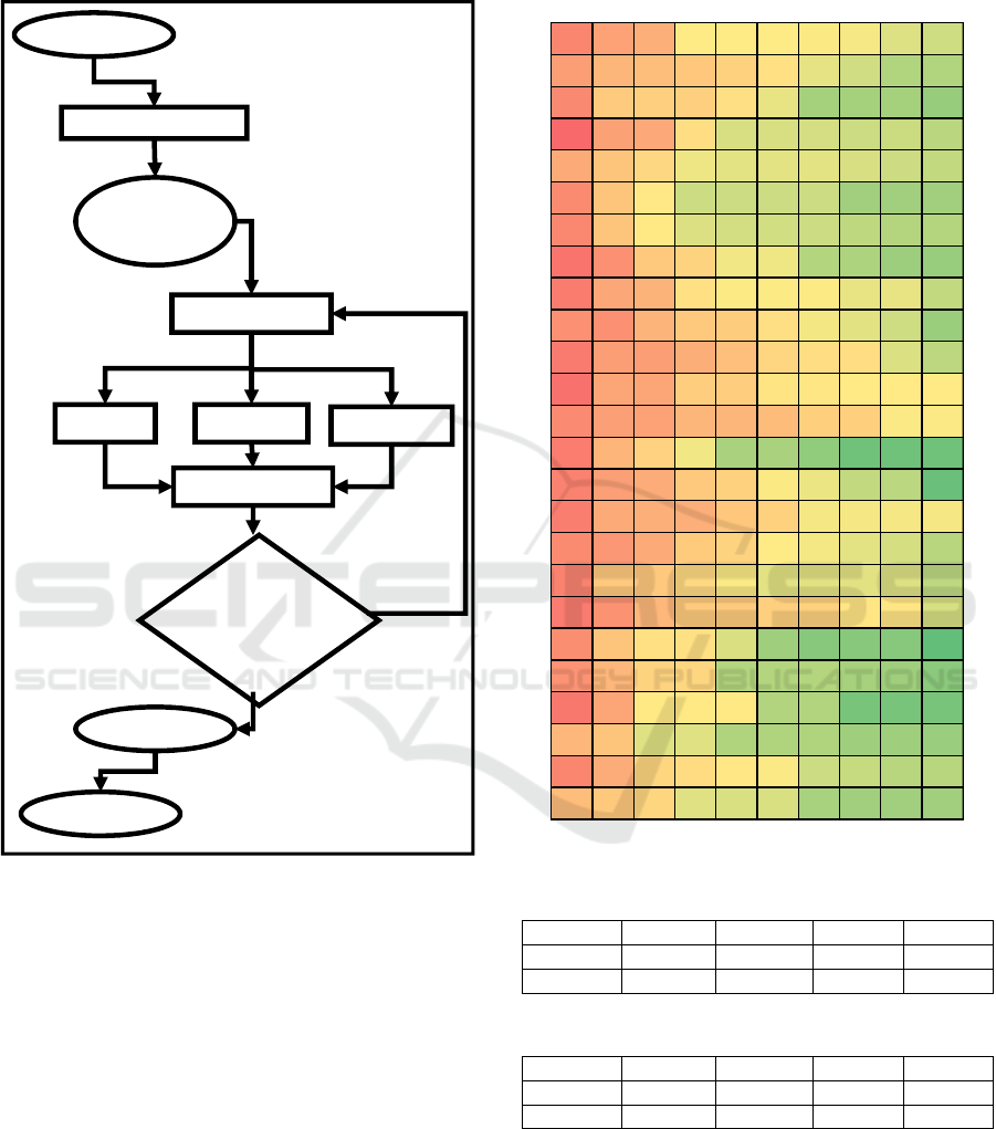
fitness function f is evaluated again. The process of
next generation formation and evaluation is repeated
for 10 times. The algorithm is repeated 25 times.
Figure 2: Genetic Programming Diagram (V. Kublanov et
al., 2017).
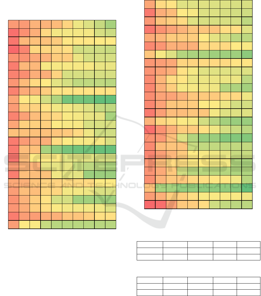
3 RESULTS
At the first step data of AP1 and ECG1 is used for
training. Data of AP2 and ECG2 is used for
validation. The results of applying the genetic
algorithm for all 25 implementations are given in
Figures 3 and 4 for Systolic (APS) and Diastolic
(APD) AP. Each line represents change of minimal
fitness function f within a single evolution. Each
column represents step of generation within a single
evolution. Different lines represent 25
implementations of genetic programming. The value
itself is the minimal value of the fitness function f for
each evolution for each generation.
Relative errors for best representatives among all
evolutions are presented in Tables 1 and 2.
Figure 3: Genetic Programming Results for APS.
Table 1: Errors for APS.
median max min std
test 8.23% 24.09% 0.62% 6.15%
validate 7.93% 33.97% 0.00% 7.68%
Table 2: Errors for APD.
median max min std
test 5.60% 26.35% 0.18% 6.71%
validate 6.32% 34.45% 0.01% 7.05%
As it can be seen, the best median results on test
data is around 8% for APS and 6% for APD. In
addition, alternative variant was considered: to the
feature vector values of HRV features of arterial
pressure on a previous segment were added. In
4,02 3,82 3,74 3,33 3,33 3,33 3,31 3,30 3,21 3,17
3,85 3,69 3,64 3,57 3,50 3,40 3,24 3,17 3,07 3,07
4,00 3,55 3,52 3,52 3,41 3,25 3,04 3,04 3,04 2,98
4,21 3,84 3,78 3,42 3,20 3,20 3,19 3,16 3,16 3,10
3,77 3,60 3,47 3,27 3,24 3,24 3,24 3,20 3,16 3,13
3,98 3,60 3,35 3,16 3,16 3,16 3,16 3,02 3,02 3,02
4,00 3,59 3,34 3,21 3,18 3,18 3,16 3,12 3,08 3,08
4,14 3,95 3,56 3,49 3,28 3,28 3,08 3,06 3,01 2,99
4,08 3,79 3,71 3,40 3,32 3,32 3,32 3,26 3,26 3,13
3,95 3,95 3,71 3,56 3,54 3,41 3,29 3,24 3,17 3,00
4,10 3,86 3,86 3,74 3,63 3,48 3,43 3,43 3,21 3,11
4,15 3,80 3,80 3,54 3,54 3,38 3,36 3,34 3,34 3,34
3,99 3,85 3,83 3,69 3,69 3,65 3,51 3,51 3,31 3,31
4,07 3,70 3,50 3,28 3,05 3,05 2,97 2,86 2,86 2,86
4,05 3,85 3,76 3,56 3,50 3,31 3,27 3,13 3,11 2,84
4,07 3,77 3,74 3,74 3,58 3,51 3,30 3,30 3,30 3,30
3,98 3,90 3,76 3,55 3,49 3,33 3,29 3,24 3,19 3,09
4,05 3,57 3,57 3,45 3,31 3,23 3,23 3,23 3,22 3,11
4,08 3,94 3,68 3,55 3,55 3,52 3,50 3,37 3,37 3,19
3,97 3,59 3,41 3,40 3,21 3,02 2,94 2,94 2,94 2,82
3,93 3,69 3,49 3,47 3,08 3,08 3,08 3,04 3,02 2,95
4,12 3,80 3,34 3,34 3,34 3,08 3,08 2,89 2,89 2,89
3,68 3,60 3,22 3,22 3,07 3,07 3,07 3,01 3,01 3,00
4,02 3,76 3,47 3,44 3,35 3,31 3,16 3,14 3,10 3,10
3,64 3,57 3,47 3,22 3,20 3,20 3,05 3,02 3,02 3,02
Start
Initial population
Start
evolution
Fitness function
Copy Crossover
Mutation
Next generation
Maximal
g
eneration is
reached?
end
end
Yes
No
Possibilities of Predicting Arterial Pressure by Means of Heart Rate Variability
351
particular AP1 and ECG1 were used for prediction of
AP2. At the same time validation was performed on
data of AP2 and ECG2 for prediction of AP3.
Results of such alternative approach are presented
on Figures 5 and 6, and on Tables 3 and 4.
Figure 4: Genetic Programming Results for APD.
It can be seen that alternative approach can
significantly improve results. It can be concluded that
task of predicting AP by means of only HRV features
can be too ambitious. At the same time the proposed
approach can be used to evaluate change in AP after
a certain time, when the original “calibration” value
is known.
It was noted that the best result was obtained for
the linear regression (polynomial of 1
st
degree). Best
combinations consist of around 20 features. Which
coupled with 1 degree lessen overtraining.
The results, presented in current work are
comparable with ones obtained using Pulsation Wave
propagation time (Anisimov et al., 2014). In that work
authors reported that for a 1/3 of validation set error
was less than 1 mmHg, average error was 9%.
Figure 5: Alternative Genetic Programming Results for
APS.
Table 3: Alternative Errors for APS.
median max min std
test 2.65% 10.07% 0.06% 2.58%
validate 4.04% 13.77% 0.00% 3.62%
Table 4: Alternative Errors for APD.
median max min std
test 4.72% 13.12% 0.05% 3.46%
validate 5.91% 21.38% 0.00% 4.84%
Results of the current work are also comparable
with results application of genetic algorithms for
symbolic regression (Dolganov, 2019). Although
additional comparison is required.
3,34 3,34 3,26 3,26 3,23 3,15 3,01 2,95 2,86 2,74
3,48 3,38 3,27 3,14 3,03 3,03 3,03 3,03 2,92 2,88
3,46 3,24 3,21 3,21 3,18 3,09 3,09 3,09 3,08 3,08
3,50 3,41 3,14 3,14 3,14 3,12 2,90 2,90 2,89 2,87
3,37 3,37 3,29 3,26 3,18 3,18 3,00 2,92 2,92 2,92
3,43 3,24 3,24 3,05 3,05 3,05 3,05 3,05 3,00 3,00
3,42 3,38 3,27 3,27 3,15 2,92 2,92 2,92 2,92 2,92
3,35 3,23 3,13 3,07 2,97 2,92 2,84 2,84 2,84 2,82
3,42 3,29 3,25 3,17 3,10 3,10 3,10 3,10 3,10 3,10
3,30 3,09 3,05 2,91 2,77 2,55 2,55 2,54 2,48 2,48
3,34 3,17 3,16 3,11 3,03 3,03 2,99 2,95 2,86 2,83
3,42 3,32 3,23 3,16 3,14 3,05 3,04 2,99 2,98 2,74
3,30 3,16 3,16 3,16 3,07 3,05 3,05 2,93 2,93 2,93
3,21 3,21 3,21 3,21 3,20 3,19 3,13 3,02 2,90 2,90
3,44 3,34 3,27 3,27 3,13 3,07 3,04 3,04 3,04 2,93
3,44 3,23 3,21 2,75 2,64 2,56 2,53 2,53 2,50 2,50
3,46 3,23 3,07 3,07 3,06 2,96 2,96 2,96 2,92 2,92
3,35 3,26 3,26 2,98 2,98 2,98 2,86 2,82 2,81 2,77
3,43 3,22 3,22 3,21 3,02 2,97 2,97 2,70 2,70 2,70
3,29 3,26 3,20 3,16 3,16 3,14 3,13 3,13 3,07 3,07
3,33 3,22 3,22 3,14 3,14 3,03 3,03 3,01 2,94 2,94
3,37 3,26 3,17 3,10 2,92 2,92 2,72 2,72 2,72 2,71
3,36 3,28 3,18 3,12 3,06 3,03 3,03 3,03 3,02 2,96
3,43 3,33 3,33 3,27 3,27 3,20 3,20 3,17 3,11 3,11
3,33 3,07 3,06 2,86 2,81 2,81 2,81 2,81 2,81 2,81
1,16 1,10 1,09 1,05 1,05 1,05 1,05 1,05 1,05 1,05
1,21 1,15 1,13 1,08 1,07 1,05 1,05 1,05 1,04 1,04
1,17 1,12 1,11 1,10 1,05 1,05 1,05 1,05 1,04 1,03
1,21 1,18 1,16 1,14 1,12 1,12 1,12 1,09 1,09 1,05
1,15 1,14 1,11 1,11 1,11 1,08 1,06 1,05 1,03 1,03
1,19 1,18 1,15 1,15 1,15 1,10 1,10 1,10 1,08 1,07
1,12 1,07 1,05 1,02 1,01 1,01 1,01 1,01 1,01 0,99
1,18 1,17 1,16 1,10 1,10 1,10 1,10 1,10 1,08 1,08
1,18 1,16 1,15 1,09 1,07 1,05 1,05 1,05 1,05 1,05
1,19 1,14 1,09 1,08 1,06 1,06 1,06 1,06 1,06 1,03
1,19 1,15 1,11 1,07 1,07 1,06 1,06 1,02 1,02 1,01
1,19 1,16 1,16 1,14 1,12 1,12 1,12 1,10 1,10 1,06
1,20 1,16 1,12 1,12 1,11 1,07 1,07 1,06 1,04 1,04
1,21 1,17 1,13 1,13 1,12 1,12 1,07 1,05 1,05 1,05
1,14 1,10 1,09 1,07 1,07 1,04 1,03 1,01 1,00 1,00
1,22 1,18 1,15 1,11 1,11 1,09 1,06 1,05 1,04 1,02
1,18 1,17 1,13 1,05 1,02 1,00 1,00 0,98 0,98 0,98
1,19 1,13 1,12 1,12 1,03 1,03 1,03 1,03 1,03 1,03
1,20 1,17 1,14 1,11 1,08 1,07 1,06 1,06 1,04 1,04
1,18 1,13 1,10 1,09 1,08 1,08 1,07 1,07 1,02 1,01
1,18 1,15 1,12 1,04 1,02 1,02 1,02 1,02 1,02 1,02
1,19 1,14 1,12 1,12 1,10 1,09 1,08 1,08 1,07 1,02
1,13 1,01 1,01 1,00 1,00 0,99 0,99 0,99 0,99 0,96
1,17 1,15 1,11 1,11 1,09 1,07 1,07 1,07 1,07 1,06
1,23 1,22 1,16 1,12 1,11 1,09 1,04 1,03 1,03 1,03
BIOSIGNALS 2020 - 13th International Conference on Bio-inspired Systems and Signal Processing
352
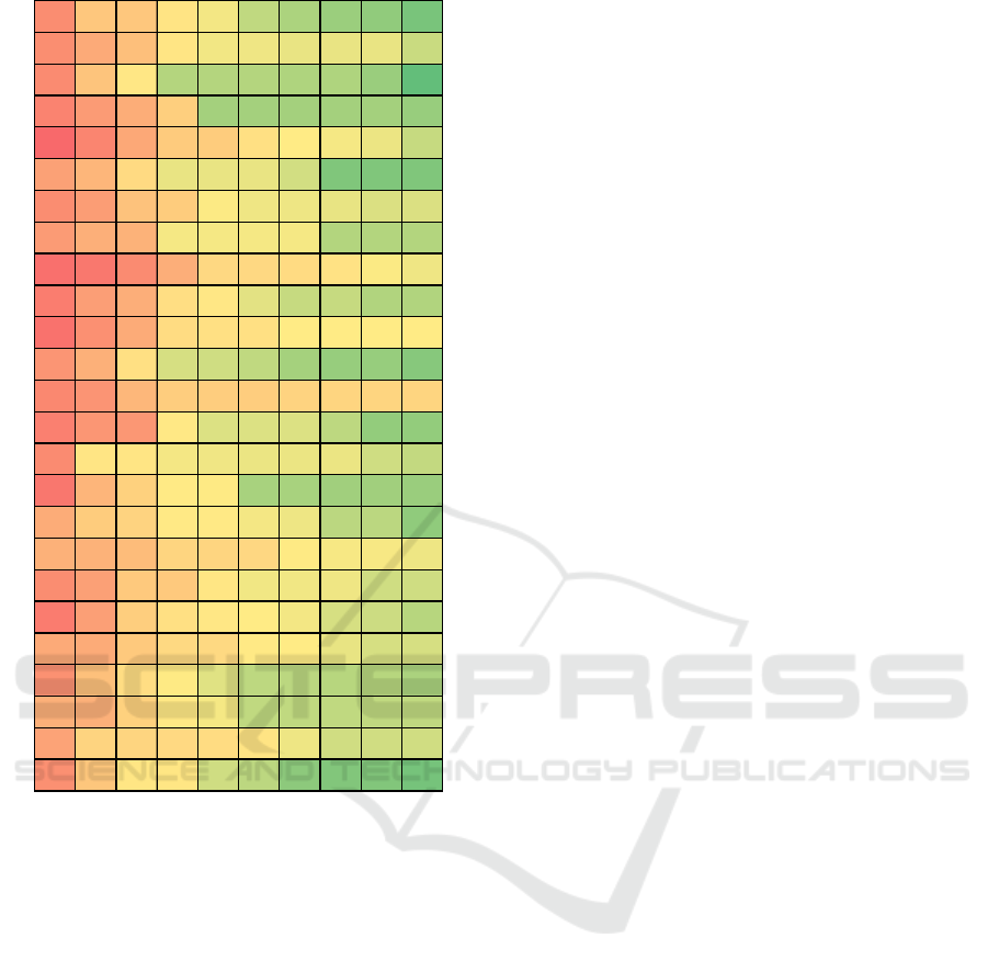
Figure 6: Alternative Genetic Programming Results for
APD.
4 DISCUSSION AND
CONCLUSIONS
The paper describes investigation testing possibility
of the indirect AP measurement by means of HRV
features. For such task a pilot study was performed on
50 student-volunteers. The study consisted of
simultaneous record of ECG signals and
measurements of AP. In the following, HRV time-
series were derived from ECG signals by software
application. A list of 64 HRV was tested.
Proposed modification of previously used
approach of genetic programming (V. Kublanov et
al., 2017).
Previously the approach was used for the
classification task in task of arterial hypertension
express-diagnosing. In the paper the approach was
modified to be applied in the regression task.
Preliminary results have shown that the error of
AP prediction using only features of HRV can be
relatively high. At the same time, when we add
“calibration” data to the HRV features it is possible
to predict change of the AP with relatively low error.
Even though the results, presented in the paper,
are relatively low, they show that there is a certain
relation between HRV features and AP data. It is
worthy to point out that no additional data was used
in current study. In particular, no data on gender,
anthropomorphic features, age was used. In addition,
features of raw ECG signals (morphology, features of
P-QRS-T complex) were also not yet tested. Addition
of such features might improve the results in the
proposed approach.
Among the possible future works directions are
application of deep neural networks (Belo et al.,
2017) in the task which proved to effective in the
biomedical signals synthesis.
REFERENCES
Addison, P. S. (2005). Wavelet transforms and the ECG: A
review. Physiological Measurement, 26(5), R155–
R199. Scopus. https://doi.org/10.1088/0967-
3334/26/5/R01
Anisimov, A. A., Yuldashev, Z. M., & Bibicheva, Yu. G.
(2014). Non-occlusion Monitoring of Arterial Pressure
Dynamics from Pulsation Wave Propagation Time.
Biomedical Engineering, 48(2), 66–69.
https://doi.org/10.1007/s10527-014-9420-7
Belo, D., Rodrigues, J., Vaz, J. R., Pezarat-Correia, P., &
Gamboa, H. (2017). Biosignals learning and synthesis
using deep neural networks. Biomedical Engineering
Online, 16(1), 115.
Dolganov, A. (2019). Indirect Measurement of Arterial
Pressure by Means of Heart Rate Variability Signals.
2019 Ural Symposium on Biomedical Engineering,
Radioelectronics and Information Technology
(USBEREIT), 156–158. https://doi.org/10.1109/
USBEREIT.2019.8736632
Egorova, D. D., Kazakov, Y. E., & Kublanov, V. S. (2014).
Principal Components Method for Heart Rate
Variability Analysis. Biomedical Engineering, 48(1),
37–41. Scopus. https://doi.org/10.1007/s10527-014-
9412-7
Kublanov, V., Dolganov, A., & Gamboa, H. (2017).
Genetic programming application for features selection
in task of arterial hypertension classification.
Proceedings - 2017 International Multi-Conference on
Engineering, Computer and Information Sciences,
SIBIRCON 2017, 561–565. Scopus. https://doi.org/
10.1109/SIBIRCON.2017.8109954
Kublanov, Vladimir, & Dolganov, A. (2019). Development
of a decision support system for neuro-
electrostimulation: Diagnosing disorders of the
1,81 1,67 1,67 1,60 1,57 1,52 1,50 1,48 1,47 1,44
1,81 1,74 1,69 1,60 1,57 1,57 1,56 1,56 1,56 1,53
1,82 1,68 1,60 1,51 1,51 1,51 1,50 1,50 1,48 1,42
1,84 1,78 1,74 1,65 1,49 1,49 1,49 1,49 1,49 1,47
1,90 1,83 1,75 1,66 1,66 1,61 1,59 1,57 1,57 1,52
1,76 1,71 1,63 1,56 1,56 1,56 1,54 1,45 1,45 1,45
1,81 1,77 1,68 1,66 1,58 1,57 1,57 1,56 1,55 1,55
1,78 1,73 1,72 1,57 1,57 1,57 1,57 1,50 1,50 1,50
1,88 1,86 1,82 1,73 1,63 1,63 1,62 1,61 1,58 1,57
1,85 1,77 1,73 1,62 1,60 1,56 1,52 1,52 1,50 1,50
1,87 1,80 1,74 1,62 1,61 1,61 1,59 1,59 1,59 1,59
1,79 1,73 1,61 1,54 1,53 1,52 1,49 1,47 1,47 1,46
1,82 1,79 1,71 1,66 1,66 1,66 1,64 1,64 1,64 1,64
1,84 1,79 1,79 1,59 1,55 1,55 1,55 1,52 1,47 1,47
1,82 1,60 1,60 1,57 1,57 1,56 1,56 1,56 1,53 1,52
1,87 1,72 1,65 1,59 1,58 1,49 1,49 1,48 1,48 1,48
1,74 1,66 1,64 1,59 1,59 1,57 1,57 1,51 1,51 1,47
1,72 1,72 1,70 1,64 1,64 1,63 1,58 1,58 1,58 1,57
1,81 1,77 1,67 1,67 1,60 1,57 1,57 1,57 1,53 1,53
1,85 1,77 1,66 1,61 1,59 1,59 1,57 1,54 1,53 1,51
1,74 1,74 1,67 1,63 1,63 1,59 1,59 1,56 1,54 1,54
1,80 1,69 1,62 1,58 1,55 1,51 1,51 1,51 1,51 1,49
1,73 1,73 1,65 1,59 1,57 1,52 1,52 1,52 1,52 1,52
1,76 1,64 1,64 1,63 1,62 1,60 1,57 1,54 1,54 1,54
1,81 1,68 1,60 1,60 1,53 1,51 1,46 1,45 1,45 1,44
Possibilities of Predicting Arterial Pressure by Means of Heart Rate Variability
353

cardiovascular system and evaluation of the treatment
efficiency. Applied Soft Computing, 77, 329–343.
https://doi.org/10.1016/j.asoc.2019.01.032
Kurylyak, Y., Lamonaca, F., & Grimaldi, D. (2013). A
Neural Network-based method for continuous blood
pressure estimation from a PPG signal. 2013 IEEE
International Instrumentation and Measurement
Technology Conference (I2MTC), 280–283. https://
doi.org/10.1109/I2MTC.2013.6555424
Malik, M. (1996). Heart rate variability: Standards of
measurement, physiological interpretation, and clinical
use. Circulation, 93(5), 1043–1065. Scopus.
Mallat, S. (2009). A Wavelet Tour of Signal Processing.
Scopus.
Sannino, G., Falco, I. D., & Pietro, G. D. (2015). Indirect
Blood Pressure Evaluation by Means of Genetic
Programming. Biomedical Engineering Systems and
Technologies, 75–92. https://doi.org/10.1007/978-3-
319-27707-3_6
Simjanoska, M., Gjoreski, M., Bogdanova, A. M., Koteska,
B., Gams, M., & Tasič, J. (2018). ECG-derived Blood
Pressure Classification using Complexity Analysis-
based Machine Learning. 282–292. https://www.
scitepress.org/PublicationsDetail.aspx?ID=I16nQUpZj
Dw=&t=1
Simjanoska, M., Papa, G., Seljak, B., & Eftimov, T. (2019).
Comparing Different Settings of Parameters Needed
for Pre-processing of ECG Signals used for Blood
Pressure Classification. 62–72. https://www.
scitepress.org/PublicationsDetail.aspx?ID=tgp8l7PfXk
w=&t=1
Stein, P. K., Bosner, M. S., Kleiger, R. E., & Conger, B. M.
(1994). Heart rate variability: A measure of cardiac
autonomic tone. American Heart Journal, 127(5),
1376–1381.
Ushakov, I. B., Orlov, O. I., Baevskii, R. M., Bersenev, E.
Y., & Chernikova, A. G. (2013). Conception of health:
Space-Earth. Human Physiology, 39(2), 115–118.
Scopus. https://doi.org/10.1134/S0362119713020175
WHO. (2018). World health statistics 2018: Monitoring
health for the SDGs sustainable development goals.
World Health Organization.
Zwillinger, D., & Kokoska, S. (1999). CRC standard
probability and statistics tables and formulae. Crc
Press.
BIOSIGNALS 2020 - 13th International Conference on Bio-inspired Systems and Signal Processing
354
