
Delay Predictors in Multi-skill Call Centers: An Empirical Comparison
with Real Data
Mamadou Thiongane
1
, Wyean Chan
2
and Pierre L’Ecuyer
2
1
Department of Mathematics and Computer Science, University Cheikh Anta Diop, Dakar, S
´
en
´
egal
2
Department of Computer Science and Operations Research, University of Montreal, Montr
´
eal QC, Canada, U.S.A.
Keywords:
Delay Prediction, Waiting Time, Automatic Learning, Neural Networks, Service Systems, Multi-skill Call
Centers.
Abstract:
We examine and compare different delay predictors for multi-skill call centers. Each time a new call (cus-
tomer) arrives, a predictor takes as input some observable information from the current state of the system,
and returns as output a forecast of the waiting time for this call, which is an estimate of the expected waiting
time conditional on the current state. Any relevant observable information can be included, e.g., the time of
the day, the set of agents at work, the queue size for each call type, the waiting times of the most recent calls
who started their service, etc. We consider predictors based on delay history, regularized regression, cubic
spline regression, and deep feedforward artificial neural networks. We compare them using real data obtained
from a call center. We also examine the issue of how to select the input variables for the predictors.
1 INTRODUCTION
In service systems such as call centers, medical clin-
ics, emergency services, and many others, announc-
ing to new arriving customers an accurate estimate
of their waiting time until the call is answered or the
service begins, immediately upon arrival, can be im-
prove the customer’s experience and satisfaction. For
first-come first-served systems with a single type of
customer and server, simple formulas are sometimes
available for the expected waiting time conditional on
the state of the system. But for more complex sys-
tems in which several types of customers share differ-
ent types of servers with certain priority rules (such as
in multi-skill call centers), computing good predictors
is generally much more difficult, because for example
there are more sources of uncertainty and the condi-
tional waiting time distribution depends on a much
larger number of variables that determine the state of
the system. For instance, we may not know which
type of server will serve this customer, higher-priority
customers may arrive before the service starts, etc.
Proposed solutions to this problem are currently very
limited.
The aim of this paper is to examine different
learning-based delay predictors for multi-skill call
centers. We compare their effectiveness using real
data collected from a multi-skill call center. The pa-
rameters of the predictors are learned from part of this
data, and the rest of the data is used to measure the ac-
curacy of these delay predictors.
Most previous work on delay estimation was for
queueing systems with a single type of customer and
identical servers. The proposed methods for this case
can be classified in two categories: queue-length (QL)
predictors and delay-history (DH) predictors. A QL
predictor estimates the waiting time of a new arriving
customer with a function of the queue length when
this customer arrives. This function generally de-
pends on system parameters. In simple cases, with
exponential service times, it may correspond to an an-
alytical formula that gives the exact expected waiting
time conditional on the current state of the system;
see, e.g., Whitt (1999); Ibrahim and Whitt (2009a,
2010, 2011). A DH predictor, on the other hand, uses
the past customer delays to predict the waiting time
of a new arriving customer (Nakibly, 2002; Armony
et al., 2009; Ibrahim and Whitt, 2009b; Thiongane
et al., 2016; Dong et al., 2018). We discuss them in
Section 2.
There has been only limited work on developing
predictors for queueing systems with multiple types
of customers and multiple queues that can share some
servers, as in multi-skill call centers, in which each
server is an agent that can handle a subset of the call
types, and each call type has its own queue. The QL
100
Thiongane, M., Chan, W. and L’Ecuyer, P.
Delay Predictors in Multi-skill Call Centers: An Empirical Comparison with Real Data.
DOI: 10.5220/0009181401000108
In Proceedings of the 9th International Conference on Operations Research and Enterprise Systems (ICORES 2020), pages 100-108
ISBN: 978-989-758-396-4; ISSN: 2184-4372
Copyright
c
2022 by SCITEPRESS – Science and Technology Publications, Lda. All rights reserved

predictors perform well in single-queue systems but
do not apply (and are very difficult to adapt) to multi-
skill systems. The DH predictors can be used for
multi-skill systems but they often give large predic-
tion errors for those systems (Thiongane et al., 2016).
Senderovich et al. (2015) proposed predictors for
a multi-skill call center with multiple call types but a
single type (or group) of agents that can handle all
call types. Thiongane et al. (2015) proposed data-
based delay predictors that can be used for more gen-
eral multi-skill call centers or service systems. The
predicting functions were regression splines (RS) and
artificial neural network (ANN), and the input state
variables were the waiting time of the last customer of
the same type to have entered service, and the lengths
of some queues. The predictors were compared em-
pirically on small and simple simulation models, but
not on real data. In a similar vein, Ang et al. (2016)
studied the lasso regression (LR) method (Tibshirani,
1999) to predict waiting times in emergency (health-
care) departments, based on input variables such as
the queue length, and functions of them. Some of
these variables correspond to QL predictors that are
not directly applicable in the multi-skill setting. Nev-
ertheless, RL can be used in multi-skill call centers as
well, with appropriate input variables. In these paper,
the RS, LR, and ANN predictors are referred to as
machine learning (ML) delays predictors. Their per-
formance will depend largely on the input variables
considered. If important variables are left out, the
forecast may lose accuracy significantly.
In this work, we compare the performances of RS,
LR, ANN, and various types of DH predictors, on real
data taken from an existing call center. The ANNs we
use are multilayer feed-forward neural networks. Our
main contributions are: (i) we propose a method to
select the relevant variables to predict the customers
wait times in multi-skill setting with the ML predic-
tors; (ii) we show the impact of leaving out some im-
portant input variables on the accuracy of ML predic-
tors; (iii) we test the accuracy of all these predictors
in a real multi-skill setting.
The remainder is organized as follows. In Section
2, we recall the definitions of various DH and ML
delay predictors. Section 3 describes the call center
and the data used for our experiments, and how we
have recovered the needed data that was not directly
available. Section 4 Numerical results are reported
and discussed in Section 5 contains a conclusion and
final remarks.
2 DELAY PREDICTORS
In this section, we briefly describe the DH and ML
delay predictors used in this work. We do not consider
the QL predictors in this work because they do not
apply in multi-skill settings.
2.1 DH Predictors
DH predictors use past customer delays to predict
the waiting time of a newly arriving customer. They
do not require a learning phase to optimize several
parameters and they are easy to implement in prac-
tice. The DH predictors considered here are the best
performers on experiments with simulated system,
among those we found in the literature. They are de-
fined as follows.
Last-to-Enter-Service (LES). This predictor re-
turns the wait time experienced by the customer of the
same class who was the last enter the system, among
those who had to wait and have started their service
(Ibrahim and Whitt, 2009b). It is the most popular
DH predictor.
Average LES (Avg-LES). This one returns the av-
erage delay experienced by the N (a fixed integer)
most recent customers of the same class who entered
service after waiting a positive time. It is often used
in practice (Dong et al., 2018).
Average LES Conditional on Queue Length
(AvgC-LES). This one returns an average of the
wait times of past customers of the same class who
found the same queue length when they arrived. It
was introduced in (Thiongane et al., 2016) and was
the best performing DH predictor in some experi-
ments with simulated systems in that paper.
Extrapolated LES (E-LES). For a new customer
of class j, this predictor use the delay information
of all customers of the same class that are currently
waiting in queue. The final wait times of these cus-
tomers are still unknown, but the elapsed (partial) de-
lays are extrapolated to predict the final delays of all
these customers, and E-LES returns a weighted av-
erage of these extrapolated delays (Thiongane et al.,
2016).
Proportional Queue LES (P-LES). P-LES read-
justs the time delay x of the LES customer to account
for the difference in the queue length seen by the LES
and the new arriving customer (Ibrahim et al., 2016).
Delay Predictors in Multi-skill Call Centers: An Empirical Comparison with Real Data
101

If Q
LES
denotes the number of customers in queue
when the LES customer arrived, and Q the number
of customers in queue ahead of the new arrival, the
waiting time of this new customer is predicted by
D = x
Q + 1
Q
LES
+ 1
.
2.2 ML Delay Predictors
The idea behind ML predictors is to approximate the
conditional expectation of the waiting time W of an
arriving customer of type k, conditional on all ob-
servable state variables of the system at that time, by
some predictor function of selected observable vari-
ables deemed important. We denote by x the values
of these selected (input) variables, and the prediction
is F
k,θ
(x) where F
k,θ
is the predictor function for call
type k, which depends on a vector of parameters θ,
which is learned from data in a preliminary training
step.
In a simple system such as a GI/M/s queue, the
relevant state variables are the number of customers
in queue, the number s of servers, and the service rate
µ. But for more complex multi-skill centers, identify-
ing the variables that are most relevant to estimate the
expected waiting time for a given customer type k can
be challenging.
In our experiments, we proceed as follows. We
first include all observable state variables that might
have an influence on the expected waiting time. Then
we make a selection by using a feature-selection
method which provides an “importance” score for
each variable in terms of its estimated predictive
power. The variables are then ranked according to
these scores, and those with sufficiently high scores
are selected. Estimating relevant predictive-power
scores for a large number of candidate variables is
generally difficult. In our work, we do this with the
Boruta feature selection algorithm (Kursa and Rud-
nicki, 2010), which was the best performer among
several feature selection algorithms compared by De-
genhardt et al. (2017).
Boruta is actually a wrapper built over the random
forest algorithm proposed by Breiman (2001), which
uses bootstrapping to generate a forest of several deci-
sion trees. In our setting, each node in a decision tree
corresponds to a selection decision for one input vari-
able. Boruta first extends the data by adding copies
of all input variables, and shuffles these variables to
reduce their correlations with the response. These
shuffled copies are called shadow features. Boruta
runs a random forest classifier on the extended data
set. Trees are independently developed on different
bagging (bootstrap) samples of the training set. The
importance measure of each attribute (i.e., input vari-
able) is obtained as the loss of accuracy of the model
caused by the random permutation of the values of
this attribute across objects (the mean decrease accu-
racy). This measure is computed separately for all
trees in the forest that use a given attribute. Then, for
each attribute, the average and standard deviation of
the loss of accuracy is computed, a Z score is com-
puted by dividing the average loss by its standard de-
viation, and the latter is used as the importance mea-
sure. The maximum Z-score among the shadow fea-
tures (MZSA) are used to determine which variables
are useful to predict the response (i.e., the waiting
time). The attributes whose Z-scores are significantly
lower than MZSA is declared “unimportant”, those
whose Z-scores are significantly higher than MZSA
as declared “important” (Kursa and Rudnicki, 2010),
and decisions about the other ones are made using
other rules.
In this study, our candidate input variables are the
queue length for all call types (r is the vector of these
queues length, and the queue length for call type T1
to T5 are named q1 to q5 respectively), the number s
of agents that are serving the given call type, the total
number n of agents currently working in the system,
the arrival time t of the arriving customer, the wait
time of the N most recently served customers of the
given call type (they are named LES1, LES2,... , and
l is the vector of these waiting times), and the wait-
ing time predicted by the DH predictors LES, P-LES,
E-LES, Avg-LES, and AvgC-LES (d the vector that
contains these predicted waiting times).
We consider three ways of defining the predic-
tor function F
k,θ
: (1) a smoothing (least-squares re-
gression) cubic spline which is additive in the input
variables (RS), (2) a lasso (linear) regression (LR),
and (3) a deep feedforward multilayer artificial neural
network (ANN). The parameter vector θ is selected
in each case by minimizing the mean squared error
(MSE) of predictions. That is, if E = F
k,θ
(x) is the
predicted delay for a “random” customer of type k
who receives service after some realized wait time W ,
then the MSE for type k calls is
MSE
k
= E[(W −E)
2
].
We cannot compute this MSE exactly, so we estimate
it by its empirical counterpart, the average squared
error (ASE), defined as
ASE
k
=
1
C
k
C
k
∑
c=1
(W
k,c
−E
k,c
)
2
(1)
for customer type k, where C
k
is the number of served
customers of type k who had to wait in queue. We will
in fact use a normalized version of the ASE, called the
ICORES 2020 - 9th International Conference on Operations Research and Enterprise Systems
102

root relative average squared error (RRASE), which
is the square root of the ASE divided by the average
wait time of the C
k
served customers, rescaled by a
factor of 100:
RRASE =
√
ASE
(1/C
k
)
∑
C
k
c=1
W
k,c
×100.
We perform this estimation of the parameter vector
θ with a learning data set that represent 80% of the
collected data. The other 20% is used to measure and
compare the accuracy of these delay predictors.
2.2.1 Regression Splines (RS)
Regression splines are a powerful class of approxima-
tion methods for general smooth functions (de Boor,
1978; James et al., 2013; Wood, 2017). Here we use
smoothing additive cubic splines, for which the pa-
rameters are estimated by least-squares regression af-
ter adding a penalty term on the function variation to
favor more smoothness. If the information vector is
written as x = (x
1
,.. .,x
D
), the additive spline predic-
tor can be written as
F
k,θ
(x) =
D
∑
d=1
f
d
(x
d
),
where each f
d
is a one dimensional cubic spline. The
parameters of all these spline functions f
d
form the
vector θ. We estimated these parameters using the
function gam from the R package mgcv (Wood, 2019).
2.2.2 Lasso Regression (LR)
Lasso Regression is a type of linear regression (Tib-
shirani, 1996; James et al., 2013; Friedman et al.,
2010) in which a penalty term equal to the sum of ab-
solute values of the magnitude of coefficients is added
before minimizing the mean squared error, to reduce
over-fitting. If the input vector is x = (x
1
,.. .,x
D
), the
lasso regression predictor can be written as
F
k,θ
(x) =
D
∑
d=1
β
d
·x
d
+ λ.
One can estimate the parameters by using the function
glmnet from the R package gmlnet (Friedman et al.,
2019).
2.2.3 Deep Feed-forward Artificial Neural
Network (ANN)
A deep feedforward artificial neural network is an-
other very popular and effective way to approxi-
mate complicated high-dimensional functions (Ben-
gio et al., 2012; LeCun et al., 2015). This type of neu-
ral network has one input layer, one output layer, and
several hidden layers. The outputs of nodes at layer l
are the inputs of every node at the next layer l +1. The
number of nodes at the input layer is equal to the num-
ber of elements in the input vector x, and the output
layer has only one node which returns the estimated
delay. For each hidden node, we use a rectifier acti-
vation function, of the form h(z) = max(0,b + w ·z),
in which z is the vector of inputs for the node, while
the intercept b and the vector of coefficients w are pa-
rameters learned by training (Glorot et al., 2011). For
the output node in the output layer (which return the
estimated delay), we use a linear activation function,
h(z) = b + w ·z, in which z is the vector of outputs
from the nodes at the last hidden layer. The (large)
vector θ is the set of all these parameters b and w, over
all nodes. These parameters are learned by a back-
propagation algorithm that uses a stochastic gradient
descent method. Many other parameters and hyper-
parameters used in the training have to be determined
empirically. For a guide on training, see Bergstra and
Bengio (2012); Bengio (2012); Gulcehre and Bengio
(2016); Goodfellow et al. (2016). To train our ANNs
(i.e., estimate the vectors θ), we used the Pylearn2
software Goodfellow et al. (2013).
3 THE CALL CENTER AND
AVAILABLE DATA
We performed an empirical study using data from a
real multi-skill call center from the VANAD labora-
tory group, located in Rotterdam, in The Netherlands.
This center operates from 8 a.m to 8 p.m from Mon-
day to Friday. It handles 27 call types and has 312
agents. Each agent has a set of skills, which cor-
responds to a subset of the call types. The routing
mechanism works as follows. When a call arrives,
the customer first interacts with the IVR (interactive
voice response unit) to choose the call type. If there is
an available agent with this skill, the call is assigned
to the longest idle agent among those. Otherwise, the
call joins an invisible FCFS (first come first served)
queue.
The call log data has 1,543,164 calls recorded
over one year, from January 1 to December 31, 2014.
About 56% of those calls are answered immediately,
38% are answered after some wait, and about 6%
abandon. In this study, we consider only the five call
types with the largest call volume. They account for
more than 80% of the total volume. Table 1 gives a
statistical summary of the arrival counts for these five
call types, named T1 to T5. It also gives the average
waiting time (AWT), average service time (AST), and
average queue size (AQS) for each one. The other call
Delay Predictors in Multi-skill Call Centers: An Empirical Comparison with Real Data
103
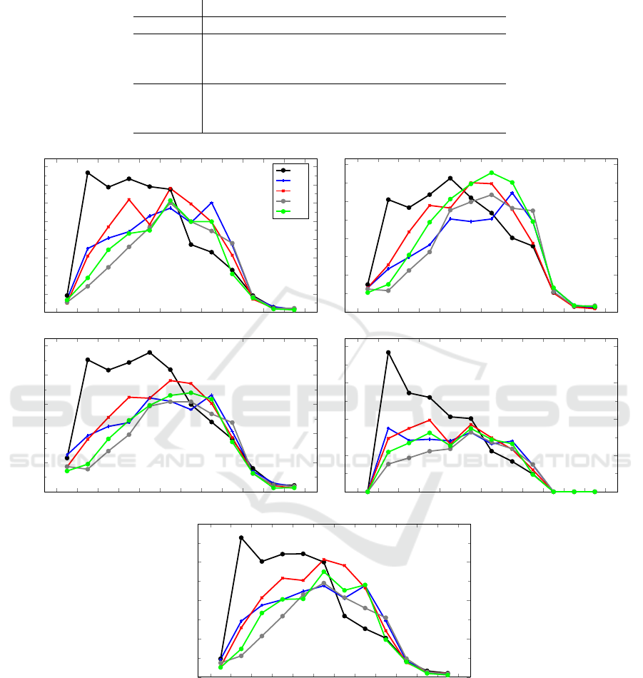
Table 1: Arrival counts and statistical summary for the five selected call types over the year. The AWT and AST
are in seconds.
T1 T2 T3 T4 T5
Number 568 554 270 675 311 523 112 711 25 839
No wait 61% 52% 55% 45% 34%
Wait 35% 40% 40% 46% 54%
Abandon 4% 7% 5% 8% 12%
AWT 77 91 83 85 110
AST 350 308 281 411 311
AQS 8.2 3.3 4.4 4.3 0.9
8 9 10 11 12 13 14
15 16
17 18 19 20
0
20
40
60
80
100
120
140
160
Period of 1 hour (call type T1)
Mean arrival counts
Mo
Th
We
Th
Fr
8 9 10 11 12 13 14
15 16
17 18 19 20
0
20
40
60
80
Period of 1 hour (call type T2)
Mean arrival counts
8 9 10 11 12 13 14
15 16
17 18 19 20
0
20
40
60
80
100
Period of 1 hour (call type T3)
Mean arrival counts
8 9 10 11 12 13 14
15 16
17 18 19 20
0
20
40
60
80
Period of 1 hour (call type T4)
Mean arrival counts
8 9 10 11 12 13 14
15 16
17 18 19 20
0
5
10
15
20
Period of 1 hour (call type T5)
Mean arrival counts
Figure 1: Average arrival counts per hour and per call type, for each type of day, over the year.
types, not considered here, accounted for less than
10 000 calls altogether during the year. Each one had
less than 30 calls a day on average. We do not study
delay predictors for them.
Figure 1 shows the average number of arrivals per
hour per call type, for each day of the week, over the
year. We see from this figure that the arrival behavior
for Monday differs significantly from that of the other
days, especially in the morning. A plausible explana-
tion for this is that Monday is the first day of the week
and the center is closed on the two previous days. This
means that it would make sense to develop two sepa-
ICORES 2020 - 9th International Conference on Operations Research and Enterprise Systems
104
0 50 100 150 200 250 300
0.000
0.002 0.004 0.006 0.008 0.010
Waiting time (sec)
Density
T1
T2
T3
T4
T5
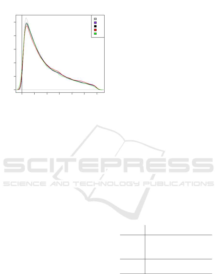
Figure 2: Waiting time density for calls who waited and
were served, per call type.
rate sets of predictors: one for Monday’s and one for
the other days. In this paper, we focus on the other
days (Tuesday to Friday). Figure 2 shows a density
estimate of the waiting time for calls who waited and
did not abandon, for the five considered call types.
These densities were estimated using kernel density
estimators with a normal kernel. This explains the
fact that part of the density near zero “leaks” to the
negative side. The true density starts at zero.
The data contains the following information on
each call received in the one-year period: the call
type, the arrival time, the date, the desired service, and
the VRU entry and exit time. There is also a queue en-
try time and a queue exit time, but only for the calls
that have to wait. For those calls, we also know if
they received service or abandoned. Finally, for the
called that were served, we have the times when ser-
vice started and when it ended, and we can easily
compute the realized waiting time of the call.
For the ML predictors, when a call arrives, we
need to observe a large number of candidate input
variables (features) in x = (r,s, n,l,d,t) that are re-
quired to predict the waiting time of this call. How-
ever, most of this information is not directly available
in the data. Similarly, much of the information re-
quired for the DH predictors is not directly observ-
able in the historical data. To address this issue, we
had to build a simulator that could replay the history
from the available data and compute all this miss-
ing information (e.g., the detailed state of the sys-
tem each time a customer arrives, the LES, Avg-LES,
etc.). This simulator was implemented in Java using
the simevent package of the SSJ simulation library
(L’Ecuyer et al., 2002; L’Ecuyer, 2016).
4 NUMERICAL EXPERIMENTS
4.1 Identifying the Important Input
Variables
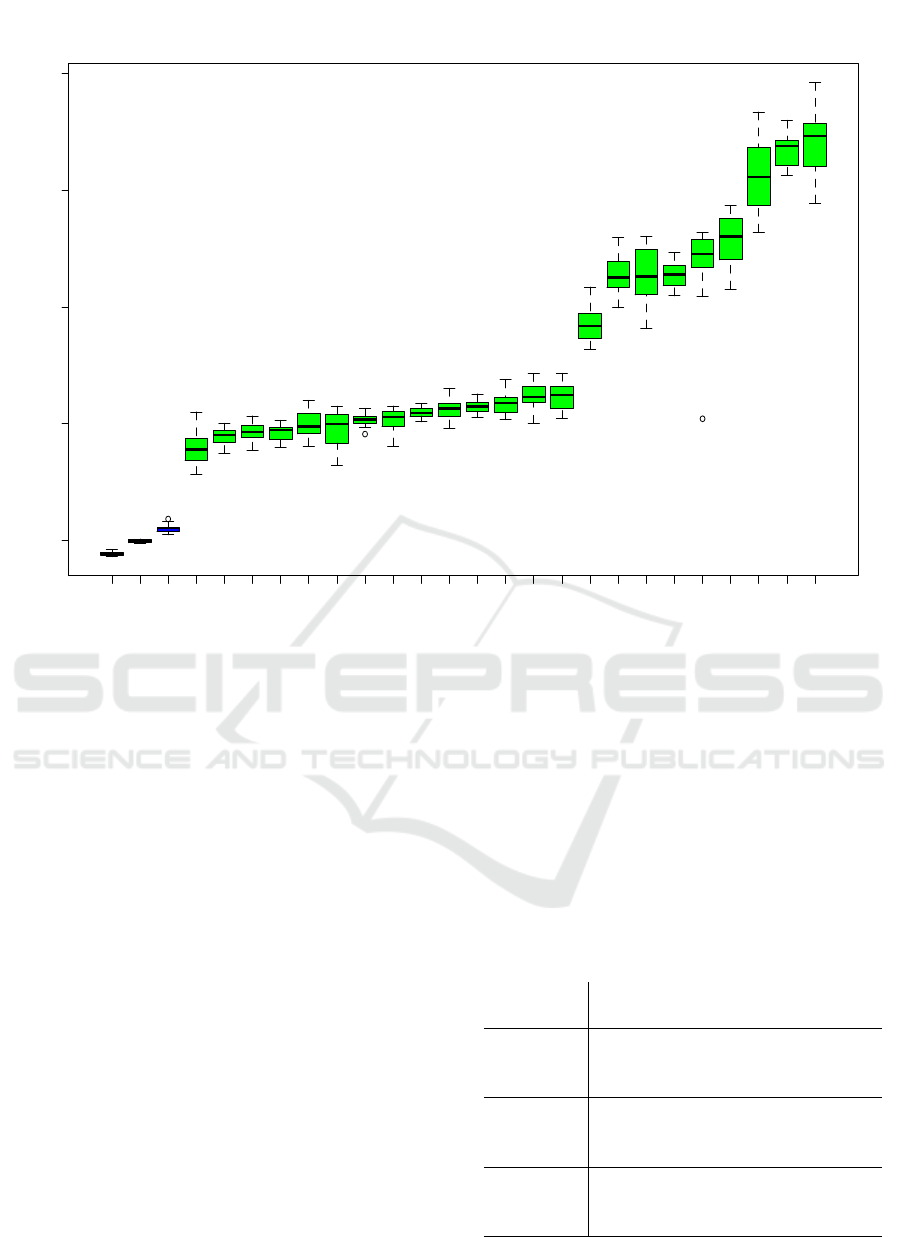
After reconstructing the detailed data, we ran the
Boruta algorithm on the data set for each call type
to identify the candidate variables that are important
to predict the waiting time. As an illustration of the
results, Figure 3 reports the importance scores of the
input variables for call type T1. It shows a box plot of
the Z-scores of all the attributes (input variables), plus
the minimum, the average, and the maximum shadow
scores. All the candidate variables have their box-
plots (in green) much higher than the shadow scores,
which means that they are all declared “important”
by Boruta. The same was observed for all other call
types.
We also see in the figure that the most important
input variables to predict waiting times (those with the
highest Z-scores) for call type T1 are (in this order)
the arrival time t of the call, the queues length, the
prediction of AvgC-LES, the total number n of agents
in the system, and the number s of agents serving this
call type. The other variables have a lower score.
We then made an experiment to see if removing all
these lower-score input variables from the selected in-
puts would make a difference in prediction accuracy,
and found no significant difference (less than 0.1% in
all cases). Therefore, we decided not to include them
as input variables when comparing our predictors (in
the next subsection).
4.2 RRASE with Delay Predictors
Table 2: RRASE of delay predictors.
Call Types
Predictors T1 T2 T3 T4 T5
Avg-LES 48.9 61.0 56.7 48.7 69.7
LES 44.3 57.7 51.8 44.5 66.1
AvgC-LES 44.3 56.5 51.6 42.4 62.4
E-LES 63.7 65.4 64.0 58.8 77.5
P-LES 71.2 70.5 71.4 68.5 80.3
RS 39.6 49.2 45.5 39.5 50.1
RL 41.5 51.5 47.1 38.5 51.7
ANN 36.1 46.2 44.8 37.7 48.7
Here we compare the different delay predictors in
terms of RRASE, for each call type. For all the ML
predictors, our vector of selected input variables was
x =(t, q1, q2, q3, q4, q5, n, s, LES, AvgC-LES). Table
2 reports the RRASEs. We find that the ML predic-
tors perform significantly better than the DH predic-
tors in all cases, and that the best performer is ANN.
Delay Predictors in Multi-skill Call Centers: An Empirical Comparison with Real Data
105
0 20 60 80
Importance
sh. Min
sh.Mean
sh. Max
E-LES
P-LES
LES9
LES10
LES6
Avg-LES
LES5
LES3
LES4
LES7
LES8
LES2
LES1
LES
s
n
AvgC-LES
q5
q1
q4
q2
q3
t
Figure 3: Box plot of score of variable importance.
Among the DH predictors, AvgC-LES is the best per-
former, and it is closely followed by LES and Avg-
LES. E-LES was the second best DH predictors in
previous experiments with simulated systems (Thion-
gane et al., 2016), but it does not perform well with
this real data. P-LES also performs very poorly.
4.3 Impact of Leaving Out Important
Input Variables
We made some empirical experiments to study the
impact of leaving out some input variables deemed
important by Boruta, for the ML predictors. In par-
ticular, we want to compare our ML predictors with
those proposed by Thiongane et al. (2015), for which
some of the input variables considered here were not
present. We first remove the arrival time t and the pre-
dicted delay with AvgC-LES from the input variables.
We name the ML predictors without these two vari-
ables as RS-2, LR-2, and ANN-2. Then, in addition
to the two previous variables, we also remove a queue
length for a call type that differs arriving call. We
name the resulting ML predictors RS-3, LR-3, and
ANN-3. Note that none of those three input variables
are included in x as input variables by Thiongane et al.
(2015).
Table 3 shows the RRASE of these “weakeaned”
predictors. We find that removing the first two fea-
tures reduces significantly the accuracy of ML pre-
dictors, and removing an additional one reduces the
accuracy further, again significantly. Thus, at least
for this call center, our ML predictors are more accu-
rate than those proposed by Thiongane et al. (2015).
This shows that the choice of input variables is very
important when building ML predictors.
Table 3: RRASE of delay predictors.
Call Types
Predictors T1 T2 T3 T4 T5
RS 39.6 49.2 45.5 39.5 50.1
LR 41.5 51.5 47.1 38.5 51.7
ANN 36.1 46.2 44.8 37.7 48.7
RS-2 41.9 52.0 47.7 40.9 52.5
LR-2 43.9 54.0 49.1 39.2 53.1
ANN-2 39.7 49.2 46.9 38.5 50.3
RS-3 42.5 53.0 47.9 41.2 52.9
LR-3 44.3 55.4 50.7 39.8 54.0
ANN-3 40.4 50.2 47.0 38.7 50.9
ICORES 2020 - 9th International Conference on Operations Research and Enterprise Systems
106

5 CONCLUSION
We have examined and compared several DH and ML
delay predictors on data from a real multi-skill call
center. We found that the ML predictors are much
more accurate than the DH predictors. Within the ML
predictors, ANN was more accurate than RS and LR,
but the latter can be trained much faster than ANN,
and could be more accurate when the amount of avail-
able data is smaller. We saw the negative impact of
leaving out relevant input variables on the accuracy
of the ML predictors, and illustrated how well Boruta
can identify the most relevant input variables. In on-
going work, we want to develop effective methods to
predict and announce not only a point estimate of the
waiting time, but an estimate of the entire conditional
distribution of the delay.
ACKNOWLEDGEMENTS
This work has been supported by grants from
NSERC-Canada and Hydro-Qu
´
ebec, and a Canada
Research Chair to P. L’Ecuyer. We thank Ger Koole,
from VU Amsterdam, who provided the data.
REFERENCES
Ang, E., Kwasnick, S., Bayati, M., Plambeck, E., and Ara-
tow, M. (2016). Accurate emergency department wait
time prediction. Manufacturing & Service Operations
Management, 18(1):141–156.
Armony, M., Shimkin, N., and Whitt, W. (2009). The im-
pact of delay announcements in many-server queues
with abandonments. Operations Research, 57:66–81.
Bengio, Y. (2012). Practical recommendations for gradient-
based training of deep architectures. Neural Net-
works: Tricks of the Trade, 7700:437–478.
Bengio, Y., Courville, A. C., and Vincent, P. (2012). Unsu-
pervised feature learning and deep learning: A review
and new perspectives. CoRR, abs/1206.5538:1–30.
Bergstra, J. and Bengio, Y. (2012). Random search for
hyper-parameter optimization. Journal of Machine
Learning Research, 13:281–305.
Breiman, L. (2001). Random forests. Machine learning,
45(1):5–32.
de Boor, C. (1978). A Practical Guide to Splines. Num-
ber 27 in Applied Mathematical Sciences Series.
Springer-Verlag, New York.
Degenhardt, F., Seifert, S., and Szymczak, S. (2017). Evalu-
ation of variable selection methods for random forests
and omics data sets. Briefings in Bioinformatics,
20(2):492–503.
Dong, J., Yom Tov, E., and Yom Tov, G. (2018). The im-
pact of delay announcements on hospital network co-
ordination and waiting times. Management Science,
65(5):1949–2443.
Friedman, J., Hastie, T., and Tibshirani, R. (2010). Regular-
ization paths for generalized linear models via coordi-
nate descent. Journal of Statistical Software, 33(1):1–
22.
Friedman, J., Hastie, T., Tibshirani, R., Narasimhan,
B., Simon, N., and Qian, J. (2019). R Pack-
age glmnet: Lasso and Elastic-Net Regularized
Generalized Linear Models. https://CRAN.R-
project.org/package=glmnet.
Glorot, X., Bordes, A., and Bengio, Y. (2011). Deep sparse
rectifier neural networks. In Gordon, G., Dunson,
D., and Miroslav, editors, Proceedings of the Four-
teenth International Conference on Artificial Intelli-
gence and Statistics, volume 15 of Proceedings of Ma-
chine Learning Research, pages 315–323, Fort Laud-
erdale, FL, USA. PMLR.
Goodfellow, I., Bengio, Y., and Courville, A.
(2016). Deep Learning. MIT Press.
http://www.deeplearningbook.org.
Goodfellow, I., Warde-Farley, D., Lamblin, P., Dumoulin,
V., Mirza, M., Pascanu, R., Bergstra, J., Bastien, F.,
and Bengio, Y. (2013). Pylearn2: A machine learning
research library.
Gulcehre, C. and Bengio, Y. (2016). Knowledge mat-
ters: Importance of prior information for optimization.
Journal of Machine Learning Research, 17:1–32.
Ibrahim, R., L’Ecuyer, P., Shen, H., and Thiongane, M.
(2016). Inter-dependent, heterogeneous, and time-
varying service-time distributions in call centers. Eu-
ropean Journal of Operational Research, 250:480–
492.
Ibrahim, R. and Whitt, W. (2009a). Real-time delay es-
timation based on delay history. Manufacturing and
Services Operations Management, 11:397–415.
Ibrahim, R. and Whitt, W. (2009b). Real-time delay estima-
tion in overloaded multiserver queues with abandon-
ments. Management Science, 55(10):1729–1742.
Ibrahim, R. and Whitt, W. (2010). Delay predictors for cus-
tomer service systems with time-varying parameters.
In Proceedings of the 2010 Winter Simulation Confer-
ence, pages 2375–2386. IEEE Press.
Ibrahim, R. and Whitt, W. (2011). Real-time delay esti-
mation based on delay history in many-server service
systems with time-varying arrivals. Production and
Operations Management, 20(5):654–667.
James, G., Witten, D., Hastie, T., and Tibshirani, R. (2013).
An Introduction to Statistical Learning, with Applica-
tions in R. Springer-Verlag, New York.
Kursa, M. B. and Rudnicki, W. R. (2010). Feature selec-
tion with the boruta package. Journal of Statistical
Software, 36:1–13.
LeCun, Y., Bengio, Y., and Hinton, G. (2015). Deep learn-
ing. Nature, 521:436–444.
L’Ecuyer, P. (2016). SSJ: Stochastic simulation in Java.
http://simul.iro.umontreal.ca/ssj/.
L’Ecuyer, P., Meliani, L., and Vaucher, J. (2002). SSJ:
A framework for stochastic simulation in Java. In
Y
¨
ucesan, E., Chen, C.-H., Snowdon, J. L., and
Charnes, J. M., editors, Proceedings of the 2002
Delay Predictors in Multi-skill Call Centers: An Empirical Comparison with Real Data
107

Winter Simulation Conference, pages 234–242. IEEE
Press.
Nakibly, E. (2002). Predicting waiting times in telephone
service systems. Master’s thesis, Technion, Haifa, Is-
rael.
Senderovich, A., Weidlich, M., Gal, A., and Mandelbaum,
A. (2015). Queue mining for delay prediction in
multi-class service processes. Information Systems,
53:278–295.
Thiongane, M., Chan, W., and L’Ecuyer, P. (2015). Waiting
time predictors for multiskill call centers. In Proceed-
ings of the 2015 Winter Simulation Conference, pages
3073–3084. IEEE Press.
Thiongane, M., Chan, W., and L’Ecuyer, P. (2016). New
history-based delay predictors for service systems. In
Proceedings of the 2016 Winter Simulation Confer-
ence, pages 425–436. IEEE Press.
Tibshirani, R. (1996). Regression shrinkage and selection
via the LASSO. Journal of the Royal Statistical Soci-
ety, Series B (Methodological), pages 267–288.
Tibshirani, R. (1999). Regression shrinkage and selection
via the lasso. Journal of the Royal Statistical Society,
7(0):267–288.
Whitt, W. (1999). Predicting queueing delays. Management
Science, 45(6):870–888.
Wood, S. N. (2017). Generalized Additive Models: An In-
troduction with R. Chapman and Hall / CRC Press,
Boca Raton, FL, second edition.
Wood, S. N. (2019). R Package mgcv: Mixed GAM Compu-
tation Vehicle with Automatic Smoothness Estimation.
https://CRAN.R-project.org/package=mgcv.
ICORES 2020 - 9th International Conference on Operations Research and Enterprise Systems
108
