3D Spatial Dependencies Study in the Hawk and Dove Model

Andrzej Swierniak

, Marek Bonk and Damian Borys

Silesian University of Technology, Faculty of Automatic Control, Electronics and Computer Science,

Akademicka 16, Gliwice, Poland

Keywords:

Evolutionary Games, Game Theory, Spatial, 3D Grid.

Abstract:

The aim of the research was to check spatial dependencies in evolutionary games in 3D grids and compare

them with simulation results (2D) and theoretical or analytical considerations obtained from the replicator

dynamics equations. In order to compare the results, the classic Hawk and Dove model was used and a series

of simulations for both v < c and v > c cases was performed using our own software. The results are almost

the same as the theoretical analysis of this model, but some small differences were observed and discussed. It

seems, however, that the 3D model better reﬂects the behaviour of the population than 2D simulations.

1 INTRODUCTION

The theory of evolutionary game theory (EGT) initi-

ated by JM. Smith and G. Price (Sigmund and Nowak,

1999; Smith, 1982) allow expressing the idea of Dar-

win’s matching of genres and their evolution with the

elegant mathematical apparatus of game theory. This

ﬁeld of knowledge has allowed the creation of meth-

ods for simulation and analysis of the dynamics of the

population of individuals observed in the biological

world. The players in those games are characterised

by strategies or phenotypes that can compete or coop-

erate to achieve their evolutionary goals. Unlike stan-

dard game theory, players are instinct-based rather

than particularly rational, and the expected outcome

of the game is a better ﬁt for the environment, thereby

gaining food, partner, or living space. In the results of

individual interactions, the population may be stable,

monomorphic or multi-morphic. This state is called

evolutionary stable, and the phenotype recognised as

an evolutionary stable strategy (ESS) cannot be re-

placed by another (Smith and Price, 1973). The EGT

methodology allows us to predict the behaviour of the

population, e.g. whether one of the strategies will

be dominant. Additional information about dynamics

can be obtained from the so-called replicator dynam-

ics equations (Hofbauer et al., 1979). Still, all this

concerns the whole population and does not allow for

the analysis of its spatial structure. The use of spatial

evolutionary game theory (SEGT) (Bach et al., 2003)

https://orcid.org/0000-0002-5698-5721

https://orcid.org/0000-0003-0229-2601

allows us to supplement the missing knowledge. Each

new state of the population is obtained by perform-

ing the following steps: updating payoffs, removing

cells, reproducing. Such models have been used e.g.

in modelling cancer development (Bach et al., 2003),

modelling inter-cellular interactions including avoid-

ance of apoptosis and production of angiogenic fac-

tors (Tomlinson and Bodmer, 1997), modelling the

production of the cytotoxic substances (Tomlinson,

1997), modelling production of growth factors (Bach

et al., 2001), invasion and metastasis (Mansury et al.,

2006), tumor-environment interactions (Gatenby and

Vincent, 2003), interaction between osteoclasts and

osteoblasts (Dingli et al., 2009), tumor-stroma in-

teraction (Gerstung et al., 2011), neighbourhood ef-

fect modelling (Krzeslak and Swierniak, 2011), resis-

tance to chemotherapy (Basanta et al., 2012a) or in-

teraction of different types of cancer (Basanta et al.,

2012b). An overview of the models can be found in

the works (Basanta et al., 2008; Swierniak and Krzes-

lak, 2013). Until now, spatial analysis has been pre-

sented and analysed only in two dimensions (Krzes-

lak and Swierniak, 2016; Swierniak and Krzeslak,

2016; Swierniak and Krzeslak, 2013; Krzeslak and

Swierniak, 2011) or the third dimension meant addi-

tional resources (Swierniak et al., 2018). To relate the

models to any real, biological population, it seems

necessary to examine spatial relationships in three-

dimensional space, analysing whether the behaviour

of the studied population will show signiﬁcant differ-

ences. In this paper, we examine the spatial model

of evolutionary games for the three-dimensional gam-

Swierniak, A., Bonk, M. and Borys, D.

3D Spatial Dependencies Study in the Hawk and Dove Model.

DOI: 10.5220/0009180102330238

In Proceedings of the 13th International Joint Conference on Biomedical Engineering Systems and Technologies (BIOSTEC 2020) - Volume 3: BIOINFORMATICS, pages 233-238

ISBN: 978-989-758-398-8; ISSN: 2184-4305

233

ing space on the example of the Hawk-Dove model

known in the literature. The results of 3D simula-

tions were compared compare them with 2D simu-

lation results and theoretical or analytical consider-

ations obtained from the replicator dynamics equa-

tions. Both cases of parameter settings (for v < c and

v > c) were taken into account in the research. The in-

ﬂuence of the choice of different settings in a spatial

game was investigated and simulations for ordinary

and mixed games (MSEG - multidimensional spa-

tial evolutionary game), proposed in (Swierniak and

Krzeslak, 2016; Krzeslak et al., 2016; Krzeslak and

Swierniak, 2016; Swierniak et al., 2016), in which

each cell contains information about the composition

of different phenotypes, were carried out. Thus, a

heterogeneous subpopulation within individual cells

is represented.

2 MATERIALS AND METHODS

The game Hawk and Dove is one of the ﬁrst evo-

lutionary models proposed by John Maynard Smith

(Smith, 1982). It includes two types of phenotypes

or behaviour: combat (Hawks) or avoidance (Doves),

within the population of a single species. This pop-

ulation is a symbolic representation of the ritual con-

ﬂicts between two different strategies that evolved in

the process of evolution.

This game has two players, and each player has

his own set of decisions, which we call strategy here.

Each pair of strategies for players will result in some

game result for each player, which we call a payoff.

These values, saved in the matrix form, can be treated

as a proﬁt or the cost of choosing a particular strat-

egy. These values can also be used to model for e.g.

Darwinians ﬁtness. The payoff matrix (presented in

general form in Table 1) has two parameters: v - the

beneﬁt of the competition and c - the cost of escala-

tion.

In this model the replicator dynamics equation is

as follows:

˙x = cx (x − 1)(x −

). (1)

For Hawk and Dove game stable polymorphism

(coexistence between all phenotypes) is deﬁned by

the following evolutionarily stable strategy (ESS):

(v/c,1 − v/c) if v < c. This conditions can be

found directly from the deﬁnition of ESS or from

the Bishop-Canning theorem (Bishop and Cannings,

1978). To achieve a stable polymorphic result v must

be less than c, otherwise the population is dominated

by Hawks. The results for this model are independent

of the initial frequencies of occurrence and the plot of

Figure 1: Result of mean-ﬁeld (replication equations) dy-

namics for v=6, c=9 (v < c) in the top and v=9, c=6 (v > c)

in the bottom.

Figure 2: Initial conditions tested for Hawk and Dove

model: random (init0), Hawks in the middle (init1), Doves

in the middle (init2).

both cases (v < c and v > c) are presented on Figure

1). Those plots are the result of solving the Equation

1. Any further plots in this work are the averaged re-

sult of simulation performed in 2D or 3D grid.

Table 1: The payoff matrix for original Hawk and Dove

model.

Phenotypes Hawk Dove

Hawk v-c 2v

Dove 0 v

In this paper, we have focused on the comparison

of 2D and 3D game results, examining the impact of

the initial condition and referring these simulations to

the plots obtained from the replicator dynamic equa-

tions. The simulations were performed for three dif-

ferent initial conditions, which also gave a different

share of particular phenotypes. These were: random

distribution of individuals in the participation of 50/50

(called by us init0), Hawks concentration in the center

of the area (as init1) and Doves concentration (init2).

All those initial conditions are presented in Figure 2.

The in-house software was created to perform

BIOINFORMATICS 2020 - 11th International Conference on Bioinformatics Models, Methods and Algorithms

234

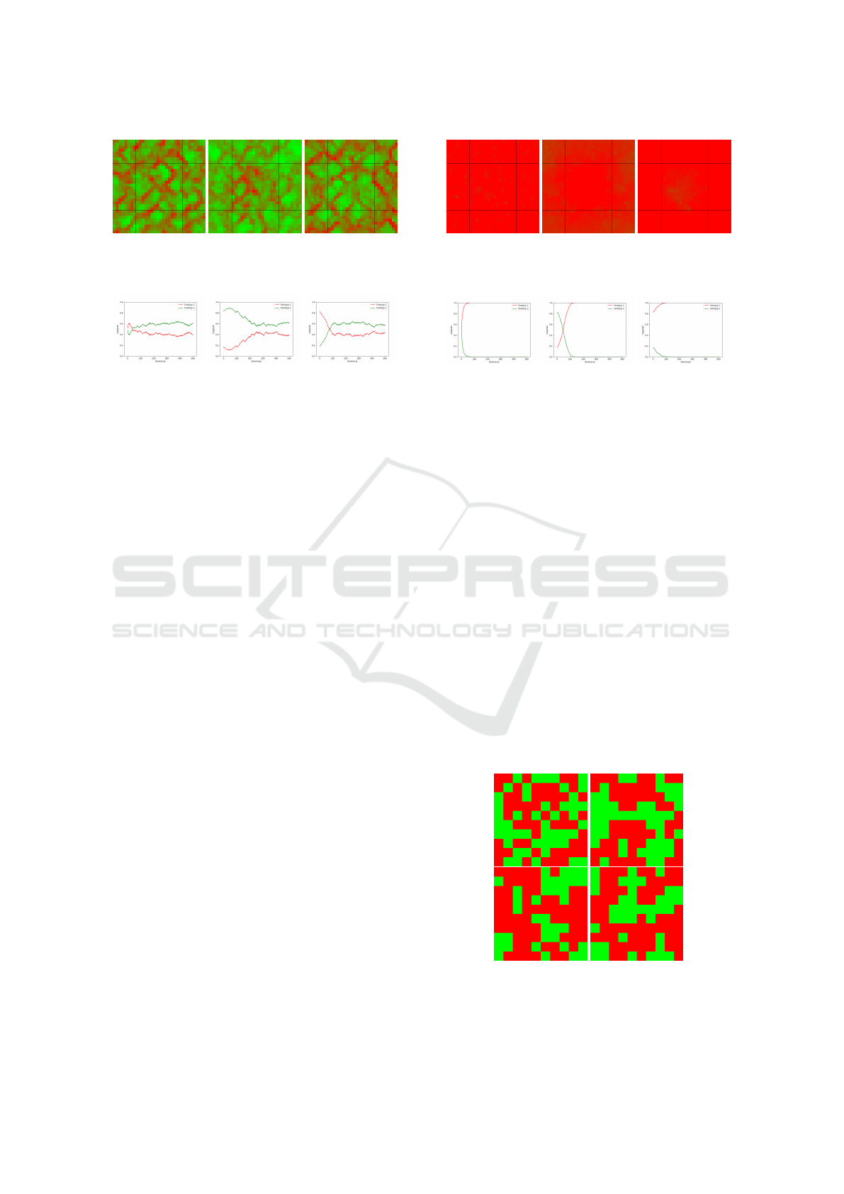
Figure 3: Result of mean 2D spatial game presented for

v=6, c=9 (v < c) and appropriately for init0, init1 and init2

conditions.

Figure 4: Averaged 2D spatial game dynamics presented in

mean-ﬁeld like plot for v=6, c=9 (v < c) and appropriately

for init0, init1 and init2 conditions.

simulations in 2D and 3D cases. Exact steps of simu-

lations were explained ﬁrst by Bach et al. (Bach et al.,

2003) and later in our previous works (Swierniak

and Krzeslak, 2013; Swierniak and Krzeslak, 2016;

Krzeslak et al., 2016; Krzeslak and Swierniak, 2016;

Swierniak et al., 2018). All simulations were per-

formed for 2D or 3D torus of size 32x32 or 10x10x10

cells. Results were analysed on spatial maps, aver-

age mean-ﬁeld like plots and averaged spatial maps.

Those averaged spatial images were analysed to show

the areas occupied by particular phenotype during the

simulation. Green colour represents Doves, and red

represents Hawks in all plots that presents the simula-

tion results.

3 RESULTS

In this section results for v=6, c=9 (v < c) and v=9,

c=6 (v > c) will be presented in Figures 3-6 for dif-

ferent initial conditions and for 2D games. Averaged

map as one in Figure 3 tells us where are areas of an

increased occurrence of a speciﬁc phenotype. For ex-

ample, pixels with almost pure red colour represents

areas where almost all the time were observed Hawks

phenotype, and vice versa - the greener the more often

Doves was in that speciﬁc location: the more mixed

colour, the more random occurrence of a speciﬁc phe-

notype.

In next section results for v=6, c=9 (v < c) are pre-

sented in Figures 7-9 for different initial conditions

and summary mean image in Figure 10.

In the last section, results for v=9, c=6 (v > c) are

presented in Figures 12-14 for different initial condi-

tions and summary mean image in Figure 15.

Figure 5: Result of mean 2D spatial game presented for

v=9, c=6 (v > c) and appropriately for init0, init1 and init2

conditions.

Figure 6: Averaged 2D spatial game dynamics presented in

mean-ﬁeld like plot for v=9, c=6 (v > c) and appropriately

for init0, init1 and init2 conditions.

4 DISCUSSION AND

CONCLUSIONS

Observation of average graphs (for example Fig. 4,

Fig. 6 etc.) allows us to state that the results of spatial

games on average overlap with theoretical considera-

tions and replicator dynamics (Fig. 1). At this level,

there were no signiﬁcant differences between 2D and

3D simulations. Only it can be noticed that for the

case v < c, where the coexistence of both popula-

tions occurs, we expected (referring to Figure 1 and

the solution of ESS) a slightly better adaptation of the

Hawks for the given parameters. However, for 2D

spatial games, the Doves phenotype showed a slightly

better adaptation. This may suggest that games sim-

ulated on 3D grids better reﬂect the behaviour of the

population. Otherwise, in the opposite case (v > c), in

each situation the results coincided with the theoreti-

Figure 7: Result of 3D spatial game presented for the mid-

dle layer for v=6, c=9 (v < c), init0 and appropriately in

generations : 0 (left-top), 50 (right-top), 200 (left-bottom)

and 500(right-bottom).

3D Spatial Dependencies Study in the Hawk and Dove Model

235

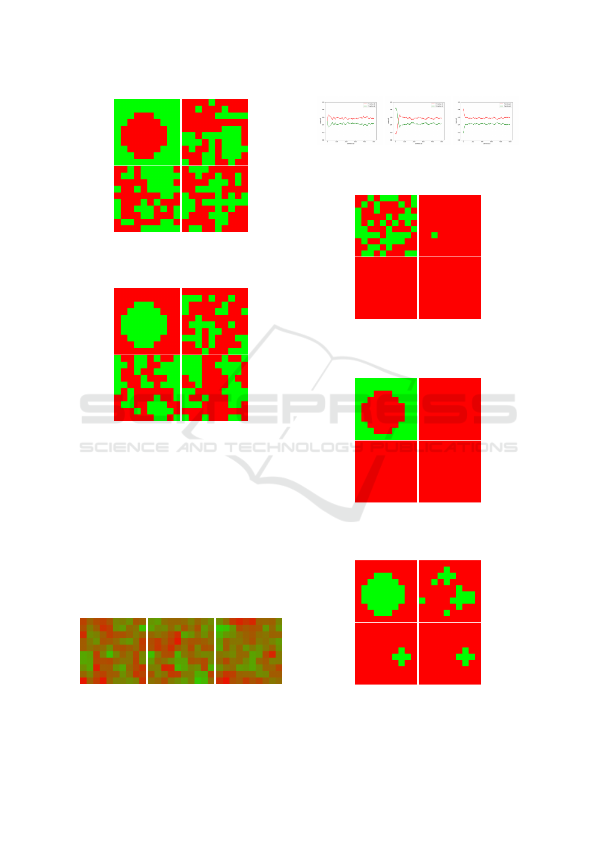
Figure 8: Result of 3D spatial game presented for the mid-

dle layer for v=6, c=9 (v < c), init1 and appropriately in

generations : 0 (left-top), 50 (right-top), 200 (left-bottom)

and 500(right-bottom).

Figure 9: Result of 3D spatial game presented for the mid-

dle layer for v=6, c=9 (v < c), init2 and appropriately in

generations : 0 (left-top), 50 (right-top), 200 (left-bottom)

and 500(right-bottom).

cal, quickly following the dominance of Hawks. The

analysis of spatial results showed that even if, in the

initial stage, the populations show some structure, the

spatial distribution quickly starts to resemble a ran-

dom one. On the average graphs in 2D, one can see a

delicate structure, where particular phenotypes were

grouped. This is not so clear for the 3D case (and

v < c), although it is possible that this is due to the

small size of the grid. An interesting structure was

observed in the results of the 3D simulations, which

seemed not to show much. After all, we expect a

Figure 10: Result of mean 3D spatial game presented for

the middle layer for v=6, c=9 (v < c) and appropriately for

init0, init1 and init2 conditions.

Figure 11: Averaged 3D spatial game dynamics presented

in mean-ﬁeld like plot for v=6, c=9 (v < c) and appropri-

ately for init0, init1 and init2 conditions.

Figure 12: Result of 3D spatial game presented for the mid-

dle layer for v=9, c=6 (v > c), init0 and appropriately in

generations : 0 (left-top), 50 (right-top), 200 (left-bottom)

and 500(right-bottom).

Figure 13: Result of 3D spatial game presented for the mid-

dle layer for v=9, c=6 (v > c), init1 and appropriately in

generations : 0 (left-top), 50 (right-top), 200 (left-bottom)

and 500(right-bottom).

Figure 14: Result of 3D spatial game presented for the mid-

dle layer for v=9, c=6 (v > c), init2 and appropriately in

generations : 0 (left-top), 50 (right-top), 200 (left-bottom)

and 500(right-bottom).

BIOINFORMATICS 2020 - 11th International Conference on Bioinformatics Models, Methods and Algorithms

236

Figure 15: Result of mean 3D spatial game presented for

the middle layer for v=9, c=6 (v > c) and appropriately for

init0, init1 and init2 conditions.

Figure 16: Averaged 3D spatial game dynamics presented

in mean-ﬁeld like plot for v=9, c=6 (v > c) and appropri-

ately for init0, init1 and init2 conditions.

quick elimination of Doves. In spatial games, it turns

out that the full elimination of Doves does not take

place, and there is always a small number of repre-

sentatives of this phenotype. What is more, on the

Figure 14 one can see a formed structure in the form

of a cross (corresponding to the settings of the sim-

ulations, i.e. Moore’s neighbourhood), where Doves

remain all the time. This trend is also clearly shown

in Figure 15 (the mean of 3D spatial game result). On

the basis of the carried out calculations, we can sug-

gest that 3D simulations seem to reﬂect the population

dynamics better, although the results are slightly more

demanding for analysis. So concluding this study we

suggest to perform spatial simulations of any game

theoretical model using 3D grids.

ACKNOWLEDGEMENTS

The study was partly supported by National Sci-

ence Centre, Poland, grant n. 2016/21/B/ST7/02241

(AS) and by Silesian University of Technology, grant

n. BK-18/0102 (DB). Calculations were performed

on the Ziemowit computer cluster in the Labo-

ratory of Bioinformatics and Computational Biol-

ogy, created in the EU Innovative Economy Pro-

gramme POIG.02.01.00-00-166/08 and expanded in

the POIG.02.03.01-00-040/13 project.

REFERENCES

Bach, L., Bentzen, S., Alsner, J., and Christiansen, F.

(2001). An evolutionary-game model of tumour-cell

interactions: possible relevance to gene therapy. Eu-

ropean Journal of Cancer, 37(16):2116–2120.

Bach, L. A., Sumpter, D. J. T., Alsner, J., and Loeschcke,

V. (2003). Spatial evolutionary games of interaction

among generic cancer cells. Journal of Theoretical

Medicine, 5(1):47–58.

Basanta, D., Gatenby, R. A., and Anderson, A. R. A.

(2012a). Exploiting evolution to treat drug resistance:

combination therapy and the double bind. Molecular

pharmaceutics, 9(4):914–21.

Basanta, D., Hatzikirou, H., and Deutsch, A. (2008). Study-

ing the emergence of invasiveness in tumours using

game theory. The European Physical Journal B,

63:393–397.

Basanta, D., Scott, J. G., Fishman, M. N., Ayala, G., Hay-

ward, S. W., and Anderson, A. R. A. (2012b). Inves-

tigating prostate cancer tumour-stroma interactions:

clinical and biological insights from an evolutionary

game. British journal of cancer, 106(1):174–81.

Bishop, D. T. and Cannings, C. (1978). A generalized war

of attrition. Journal of theoretical biology, 70(1):85–

124.

Dingli, D., Chalub, F. A. C. C., Santos, F. C., Van Seg-

broeck, S., and Pacheco, J. M. (2009). Cancer pheno-

type as the outcome of an evolutionary game between

normal and malignant cells. British journal of cancer,

101(7):1130–6.

Gatenby, R. A. and Vincent, T. L. (2003). An evolu-

tionary model of carcinogenesis. Cancer research,

63(19):6212–20.

Gerstung, M., Eriksson, N., Lin, J., Vogelstein, B., and

Beerenwinkel, N. (2011). The temporal order of ge-

netic and pathway alterations in tumorigenesis. PloS

one, 6(11):e27136.

Hofbauer, J., Schuster, P., and Sigmund, K. (1979). A note

on evolutionary stable strategies and game dynamics.

Journal of Theoretical Biology, 81(3):609–612.

Krzeslak, M., Borys, D., and Swierniak, A. (2016). An-

giogenic switch - mixed spatial evolutionary game ap-

proach. Intelligent Information and Database Sys-

tems, 9621:420–429.

Krzeslak, M. and Swierniak, A. (2011). Spatial evolu-

tionary games and radiation induced bystander effect.

Archives of Control Sciences, 21(2).

Krzeslak, M. and Swierniak, A. (2016). Multidimensional

extended spatial evolutionary games. Computers in

biology and medicine, 69:315–27.

Mansury, Y., Diggory, M., and Deisboeck, T. S. (2006).

Evolutionary game theory in an agent-based brain tu-

mor model: exploring the ’genotype-phenotype’ link.

Journal of theoretical biology, 238(1):146–56.

Sigmund, K. and Nowak, M. A. (1999). Evolutionary game

theory. Current Biology, 9(14):R503–R505.

Smith, J. M. (1982). Evolution and the theory of games.

Smith, J. M. and Price, G. R. (1973). The logic of animal

conﬂict. Nature, 246:15–18.

Swierniak, A. and Krzeslak, M. (2013). Application

of evolutionary games to modeling carcinogenesis.

Mathematical biosciences and engineering : MBE,

10(3):873–911.

3D Spatial Dependencies Study in the Hawk and Dove Model

237

Swierniak, A. and Krzeslak, M. (2016). Cancer heterogene-

ity and multilayer spatial evolutionary games. Biology

direct, 11(1):53.

Swierniak, A., Krzeslak, M., Borys, D., and Kim-

mel, M. (2018). The role of interventions in the

cancer evolution-an evolutionary games approach.

Mathematical biosciences and engineering : MBE,

16(1):265–291.

Swierniak, A., Krzeslak, M., Student, S., and Rzeszowska-

Wolny, J. (2016). Development of a population of

cancer cells: Observation and modeling by a mixed

spatial evolutionary games approach. Journal of theo-

retical biology, 405:94–103.

Tomlinson, I. (1997). Game-theory models of interactions

between tumour cells. European Journal of Cancer,

33(9):1495–1500.

Tomlinson, I. and Bodmer, W. (1997). Modelling the conse-

quences of interactions between tumour cells. British

Journal of Cancer, 75(2):157–160.

BIOINFORMATICS 2020 - 11th International Conference on Bioinformatics Models, Methods and Algorithms

238