Metagenomic Clustering in Search of Common Origin

Jolanta Kawulok and Michal Kawulok

Institute of Informatics, Silesian University of Technology, Gliwice, Poland

Keywords:

Metagenome, Metagenomic Reads, Hierarchical Clustering, Urban Microbiome, k-mers.

Abstract:

Analysis of metagenomic samples is aimed at extracting relevant information on these samples, including their

composition and origin. To determine where a sample comes from, it is commonly compared with a set of

reference samples extracted from known locations. However, if such reference samples are unavailable or

when the origins of the investigated samples are not covered by the reference set, it may be helpful to identify

groups of similar samples that may have a common origin. In this paper, we tackle this problem with hierar-

chical clustering applied to analyse a matrix of mutual similarities obtained using the Mash and our CoMeta

programs. We report initial, yet encouraging results of our experimental study performed for the metagenomic

data extracted from two large metropolises, downloaded from the Sequence Read Archive repository. The ob-

tained results indicate that the proposed approach is effective, which justiﬁes further exploration of the topic

using more extensive data.

1 BACKGROUND

In recent years, analysis of metagenomic reads (col-

lections of genome fragments derived from microbes

living in a given location) has become a hot research

topic. Such analysis has a large potential, as it is

no longer necessary to isolate and culture organisms

in laboratory conditions to study them (Simon and

Daniel, 2011; Handelsman, 2004). The majority of

the research works are aimed at discovering the com-

position of the metagenomic samples. They consist

in identifying the species of the organisms (taxonomic

classiﬁcation) or in determining the functions that can

be performed by the microorganisms from the sample

(functional classiﬁcation) (Bengtsson-Palme, 2018).

There are many metagenomic software tools for 16S

analysis and shotgun metagenomic analysis (Oulas

et al., 2015). The latter data can be analyzed follow-

ing two kinds of methodological approaches: read-

based and assembly-based (Breitwieser et al., 2017).

Metagenomic reads may also be subject to binning

(Li et al., 2012; Wang et al., 2015), which commonly

consists in clustering the reads. This process is aimed

at identifying artiﬁcial duplicates or grouping simi-

lar sequences into species or operational taxonomic

units.

Furthermore, metagenomic analysis can be used

to predict the place where the samples come from

and to create a proﬁle of that place. Walker et al.

(2018) used the 16S gene proﬁle for taxonomic clas-

siﬁcation prior to building the city proﬁles. Taxo-

nomic analysis for classifying samples to the most

probable environment was proposed by Qiao et al.

(2018), whose MetaBinG2 program allows for de-

composing the complete genome sequence into short

substrings composed of k symbols (k-mers). The use

of functional classiﬁcation was explored by Casimiro-

Soriguer et al. (2019) and Zhu et al. (2019). Zolfo

et al. (2018) used both taxonomic and functional clas-

siﬁcation for this purpose. For the metagenomic clas-

siﬁcation, various machine learning techniques are

also tested, including random forests, linear discrim-

inant analysis, and support vector machines (Harris

et al., 2019; Walker and Datta, 2019).

The aforementioned research works were focused

on comparing the query samples with those extracted

from known locations. In addition to that, dimension-

ality reduction techniques, including principal com-

ponent analysis and t-distributed stochastic neighbor

embedding, were employed to visualize the relation

between the samples based on their identiﬁed species

or functions (treated as highly-dimensional features

of these samples).

In this paper, we are focused on clustering the

metagenomic samples to identify those that may have

a common origin. Recently, we investigated such an

unsupervised scenario (Kawulok et al., 2019) with

no reference samples available, and we exploited our

218

Kawulok, J. and Kawulok, M.

Metagenomic Clustering in Search of Common Origin.

DOI: 10.5220/0009177702180225

In Proceedings of the 13th International Joint Conference on Biomedical Engineering Systems and Technologies (BIOSTEC 2020) - Volume 3: BIOINFORMATICS, pages 218-225

ISBN: 978-989-758-398-8; ISSN: 2184-4305

CoMeta program (Kawulok and Deorowicz, 2015) to

determine mutual similarities between the samples. In

our earlier research (Kawulok and Kawulok, 2018),

we demonstrated that CoMeta can be successfully

used to classify the samples by comparing them with

entire metagenomic collections derived from refer-

ence samples, which allowed us to determine their

origin. Contrary to other approaches, we proposed

to compare the metagenomic samples by measuring

their similarity directly in the space of the reads,

which means that it is not necessary to identify the

species of organisms that are present in the samples to

compute their similarity—hence a reference database

with species or functions of microorganisms is not re-

quired. After obtaining the mutual similarities, we

formed the groups of similar samples manually. The

metagenomic samples are a mixture of diverse DNA

fragments. Thus, for a number of samples derived

from several different locations, it may be expected

that appropriate clustering would help identify those

that come from the same location.

Compared to our earlier research (Kawulok et al.,

2019), here we perform automatic (rather than man-

ual) clustering of the samples to determine those that

have a common origin. For this purpose, we employ

hierarchical clustering (Rokach and Maimon, 2005)

(its important advantage is that it does not require the

number of clusters to be provided in advance), and

we consider two different approaches toward analyz-

ing the similarity matrix. Furthermore, in addition to

using CoMeta, we also exploit the Mash program to

determine the similarities between the samples. The

reported results indicate that the clusters can be cor-

rectly identiﬁed in an automatic way without the ne-

cessity of performing taxonomic or functional classi-

ﬁcation.

2 MATERIALS AND METHODS

2.1 Metagenomic Data

In our experiments, our intention was to verify, if

we could cluster the samples, even if their origins

are geographically similar to each other. There-

fore, we aimed at selecting samples extracted from

large cities located relatively close to each other, in

which there are many travellers carrying microbes

from other places. From the Sequence Read Archive

repository

(SRA), we selected two projects that pro-

vide data of urban metagenome. The ﬁrst dataset was

derived from New York City MTA subway (Afshin-

https://www.ncbi.nlm.nih.gov/sra

nekoo et al., 2015). For our experiments, we have

chosen 100 samples from them, each of which con-

tains 0.8 − 11.7 million paired-end reads (together

105.2G bases). The dataset from the second project

contains sequences from train cars and subway sta-

tions across the Boston subway system (Hsu et al.,

2016). For our experiments, we used 23 samples,

each of which contains 0.9 − 58.6 million paired-end

reads with 102 bp length.

2.2 Data Preprocessing

The SRA repository stores raw sequencing data,

therefore it can be expected that the samples ac-

quired from various cities contain highly-similar frag-

ments of the human genome. Therefore, we re-

moved human DNA from the investigated samples.

The GRCh38 latest genomic.fna.gz ﬁle (containing

human reference genome) was downloaded from the

NCBI Website. We ﬁlter each metagenome sample

using the kmc tools software (Deorowicz et al., 2015)

—if at least one human k-mer (k = 24) appears in a

read, then that read is removed from the sample.

2.3 Research Methodology

The clustering of the metagenomic samples is per-

formed on the basis of their mutual distances. For

determining the distances between the samples, we

have considered two programs.

The ﬁrst one is the Mash program which estimates

the similarity between two genomes or metagenomes.

The program uses the MinHash dimensionality re-

duction technique to compress k-mer sets of whole

genomes (Ondov et al., 2019). In the program, the

reads in the sample (S) must be ﬁrst sketched with s

hashes (s is termed the sketch size). Then, the simi-

larity between two samples is determined using these

sketched ﬁles by counting the number of overlapping

k-mers among all the s hashes.

Apart from Mash, we also used the our CoMeta

program to determine the similarities between the

samples. First, CoMeta creates k-mer databases for

all the reference samples that the query sample is to

be compared against. Subsequently, each read derived

from a query sample is compared against each other

sample (represented by a k-mer database). For each

ith read and jth sample, their similarity is computed

as the number of the nucleotides in the k-mers which

are present both in the read and in the database (asso-

ciated with that sample), divided by the length of the

query read. For clustering, a k-mer database must be

built for every sample, and then the similarity of each

sample (treated as a set of reads) to other sample (rep-

Metagenomic Clustering in Search of Common Origin

219

Comparison using CoMeta or Mash

Removal of human DNA from the

samples using the kmc tools software

— SIMS

SIMS

. . . SIMS

SIMS

— SIMS

. . . SIMS

SIMS

— . . . SIMS

SIMS

. . . —

Hierarchical clustering

Grouping of the most similar samples

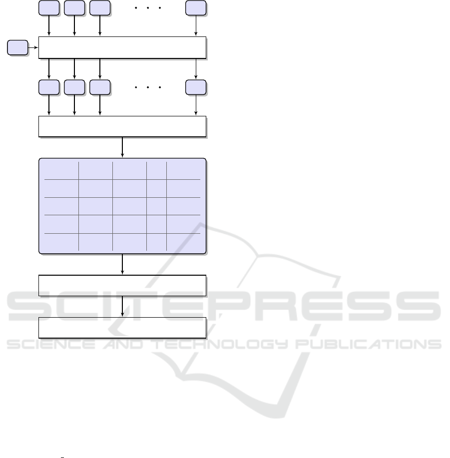
Figure 1: The processing pipeline for metagenomic reads

clustering.

resented by a k-mer database) is determined as a sum

of single-read similarities.

A simpliﬁed diagram of our clustering scheme is

shown in Figure 1. At the beginning (as described

in Section 2.2), the human fragments (S

) are sub-

tracted from the original metagenomic samples (S

)

using the kmc tools software. As a result, we ob-

tain N samples (S

) which are smaller than the orig-

inal ones. The next step is to compare the samples

between each other using CoMeta or Mash. From

these comparisons, we build a square matrix of sim-

ilarities (SSM) between the samples. It is worth not-

ing that the Mash program compares the samples us-

ing two sketched ﬁles, therefore the similarity is sym-

metrical (SIMS

= SIMS

). Contrary to that, the

CoMeta algorithm compares each sample in a read-

wise manner to a k-mer database built from another

sample. Hence, the similarities are not symmetrical

(SIMS

6= SIMS

The Mash program sketches each ﬁle using the

same size of a sketch, so despite the fact that the

ﬁles with reads are of different sizes, the size of each

sample is the same after sketching. The CoMeta pro-

gram builds a k-mer database using the whole sample,

therefore the sizes of these databases differ signiﬁ-

cantly from each other. In the reported research, we

test CoMeta program using whole k-mer databases

and using reduced databases. The latter are built af-

ter reducing each sample to the size of 0.8 million

paired-end reads (which is the size of the smallest

sample), therefore each sample is represented by a k-

mer database of the same size.

For each sample, we obtain a set of N similari-

ties between that sample and the remaining samples.

However, the distributions of the similarity values dif-

fer signiﬁcantly for individual samples. This is par-

ticularly visible for the scores obtained with CoMeta,

where even the values of self-similarity (i.e., the simi-

larity between the sample and a k-mer database cre-

ated from that sample) are varied. To address that

problem, we normalize the similarities in the follow-

ing way. First, we substitute each value on the di-

agonal (which contains the self-similarities) with the

highest value from the given row:

SIMS

← max{SIMS

: i, j ∈ h1,Ni,i 6= j}. (1)

Subsequently, each value in the row is divided by that

highest value to obtain the distance (DST) between the

samples:

DSTS

= 1 − SIMS

/SIMS

: i,k ∈ h1,Ni. (2)

In this way, we convert the SSM matrix into the

square distance matrix (SDM). While for CoMeta we

always exclude the self-similarities (1), we treat it as

an optional step for Mash, considering two versions

here: with self-similarities (WSS) and after excluding

self-similarities (ESS).

The distance matrix is subsequently used to iden-

tify the groups of samples which are supposed to have

the same origin. We consider two variants of ex-

ploiting the hierarchical clustering, namely: (origi-

nal dst)—the distances from the SDM are used as

an input for clustering; (recomputed dst)—the values

in columns are treated as individual attributes for the

samples in the rows (hence each sample is represented

with an N-dimensional feature vector containing the

distances of that sample to all the samples). In the lat-

ter variant, the Euclidean distances between the sam-

ples’ feature vectors are treated as the distances be-

tween the samples, which forms a new SDM that is

subject to hierarchical clustering.

Then, the samples are grouped using hierarchi-

cal clustering analysis (HCA). The HCA algorithm

starts by treating each sample as a singleton clus-

ter. Then, the following two steps are repeatedly exe-

cuted: (1) determine a pair of the closest clusters, and

BIOINFORMATICS 2020 - 11th International Conference on Bioinformatics Models, Methods and Algorithms

220

CoMeta (whole kmer db)

BOS

100

CoMeta (reduced kmer db )

BOS

100

(a) (b)

Mash (WSS)

BOS

100

200

300

400

500

600

700

800

900

1000

Mash (ESS)

BOS

100

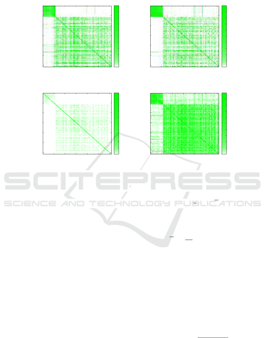
Figure 2: The square matrices of similarities between the samples.

(2) merge them together. This searching-and-merging

process is continued until all the clusters (samples)

are merged together. The relationship between the

clusters is represented by the dendrogram plot of the

hierarchical binary cluster tree. In our work, for deter-

mining the distances between sets of samples, we use

single-linkage clustering criteria, which is the shortest

distance.

3 EXPERIMENTAL VALIDATION

Our experimental study was performed using two pro-

grams: CoMeta and Mash. For the CoMeta pro-

gram, we use whole k-mer databases and reduced k-

mer databases, as explained earlier in this paper. The

SSM matrix is normalized for both programs, and for

Mash we report the results obtained without and with

excluding the self-similarities. For HCA, we use orig-

inal SDM, as well as the recomputed distance matrix.

3.1 Evaluation of Clustering

The clustering outcome can be evaluated taking into

account internal or external criteria (Rokach and Mai-

mon, 2005). As an internal quality criterium, for

M clusters, we use a sum of squared error (SSE):

D =

∑

m=1

, (3)

where N

= |C

| is the number of instances (here,

samples) belonging to the cluster C

, and:

∑

∈C

), (4)

where d(S

) is the distance between the samples S

and S

The external quality criteria can be useful for ex-

amining whether the structure of the clusters matches

some predeﬁned classiﬁcation of the samples. One

of the simplest metrics here is the Rand index, which

consists in determining the ratio between matched

and unmatched observations among two clustering

structures—C1, which is an induced clustering struc-

ture and C2, which is a given (ground-truth) clustering

structure. This index is deﬁned as:

RAND =

a + d

a + b + c + d

, (5)

where a is the number of pairs of samples that are

assigned to the same cluster in both structures (C1 and

C2); b is the number of pairs of samples that are in the

Metagenomic Clustering in Search of Common Origin

221

Samples

100

150

200

Distance

CoMeta (whole kmer db, original dst)

Samples

100

200

300

400

500

Distance

CoMeta (whole kmer db, recomputed dst)

(a) (b)

Samples

100

150

200

250

300

Distance

CoMeta (reduced kmer db, original dst)

Samples

500

1000

1500

Distance

CoMeta (reduced kmer db, recomputed dst)

Samples

1200

1250

1300

1350

1400

Distance

Mash (WSS, original dst)

Samples

1700

1750

1800

1850

1900

1950

Distance

Mash (WSS, recomputed dst)

(e) (f)

Samples

100

150

200

250

300

Distance

Mash (ESS, original dst)

Samples

200

400

600

800

1000

1200

Distance

Mash (ESS, recomputed dst)

(g) (h)

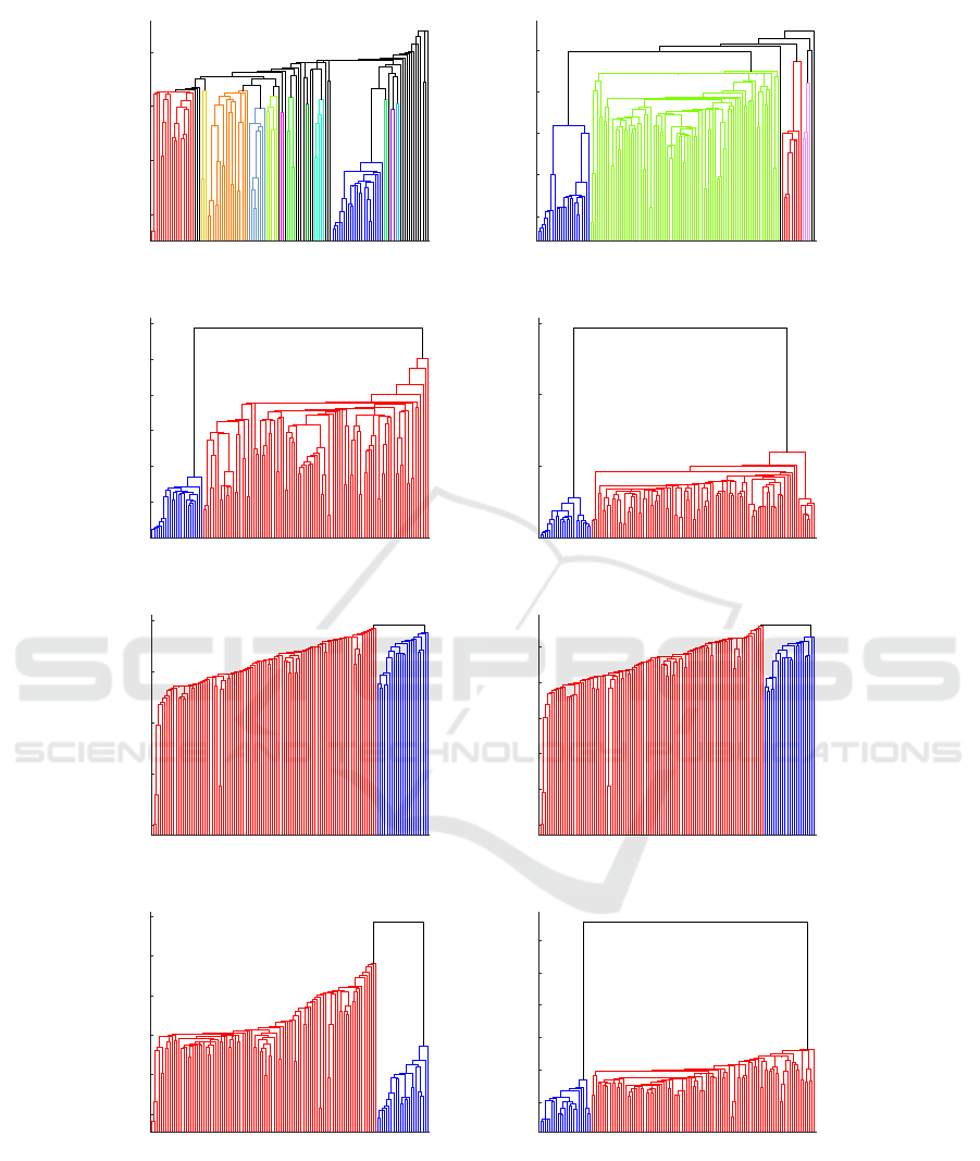
Figure 3: The dendrogram plots for hierarchical clustering. The dark blue color indicates the samples from Boston, the other

colors indicate the samples from New York.

same cluster in C1, but not in the same cluster in C2;

c is the number of pairs of samples that are in the same

cluster in C2, but not in the same cluster in C1; and

d is the number of pairs of samples that are available

in different clusters in C1 and C2. The Rand index

value lies between 0 and 1, and it equals 1 when the

samples are perfectly separated.

In addition, we inspect the appearance of the ob-

BIOINFORMATICS 2020 - 11th International Conference on Bioinformatics Models, Methods and Algorithms

222

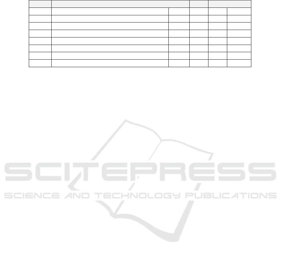
Table 1: The clustering quality scores. D

BOS

and D

are cluster-wise SSEs (4), computed for individual clusters of Boston

and New York samples, respectively; D is the overall SSE (3); and RAND is the Rand index (5). The three best scores in each

column are bolded.

Fig 3: Name: D

BOS

D RAND

(a) CoMeta (whole kmer db, original dst) 0.23 0.44 0.33 0.68

(b) CoMeta (whole kmer db, recomputed dst) 0.09 0.23 0.16 0.68

(d) CoMeta (reduced kmer db, recomputed dst) 0.08 0.23 0.15 1.00

(e) Mash (WSS, original dst) 0.47 0.49 0.48 1.00

(f) Mash (WSS, recomputed dst) 0.45 0.47 0.46 1.00

(g) Mash (ESS, original dst) 0.26 0.34 0.30 1.00

(h) Mash (ESS, recomputed dst) 0.12 0.22 0.17 1.00

tained SSM matrices and dendrograms, taking into

account how the classes are separated—we assess

whether it is easy to separate the individual clusters

based on the graphs.

3.2 Results and Discussion

Figure 2 shows the square matrixes of similarities be-

tween the samples for various cases. The results for

samples from Boston are shown in the top left cor-

ner, and it can be seen that in all cases two clusters

are formed, and they correspond with the ground truth

(i.e., with the Boston and New York samples). How-

ever, on the plot obtained with CoMeta using a whole

database (Figure 2(a)), two additional clusters can be

noticed in the bottom right corner. For Mash, ex-

cluding the self-similarities (Figure 2(d)) allowed for

strengthening the scores, and the clusters appear to be

visually better than when obtained with CoMeta.

Figure 3 shows dendrogram plots for hierarchi-

cal clustering obtained from four SDMs from Fig-

ure 2. Two methods of providing the distance matrix

to HCA were investigated—the original matrix (orig-

inal dst) and a modiﬁed matrix (recomputed dst). The

dendrograms in the left column in Figure 3(a, c, e, g)

were obtained from original distance matrices, and in

the right column (b, d, f, h) using the recomputed ma-

trices. The dark blue color indicates the samples from

Boston, and the red color indicates the samples from

New York. In the dendrograms (a, b), some additional

clusters are visible (presented with different colors in

the plots)—they show the results retrieved with the

CoMeta program, when the whole k-mer databases

are used. The dendrograms (c, d) are built using the

reduced k-mer databases in CoMeta algorithm which

balances the size of the samples. In Figure 3(g, h), the

dendrograms show the outcome obtained with Mash

after excluding the self-similarities from the SSM ma-

trix, while the dendrograms (e, f) present the results

obtained with the self-similarities.

The clustering quality scores obtained using data

shown in Figure 3 are reported in Table 1. The SSE

is the sum of squared error deﬁned in (3). It is com-

puted using additional minimum variance criteria (4),

whose values for single clusters are D

BOS

and D

for Boston and New York, respectively. The smaller

the value is, the greater is the homogeneity within the

cluster. RAND is the Rand index deﬁned in (5). The

best scores for each parameter are bolded.

Analyzing all plots, we can observe that the use

of small k-mer databases as opposed to the whole

ones allows for correct identiﬁcation of clusters for

the CoMeta program. When whole k-mer databases

are used, then some additional clusters are induced

within the New York samples which can be seen in

Figures 2(a) and 3(a, b). Hence, for these two sets of

data, the value of Rand index is below 1 in Table 1.

This means that unbalanced samples lead to identify-

ing false positive clusters in the results.

From the plots obtained for Mash, we can notice

that excluding the self-similarities allows us to sepa-

rate the samples from both cities more clearly. This

could also be noticed in Table 1—the values of D

BOS

and SSE are smaller for the Mash data after ex-

cluding the self-similarities. For more sophisticated

data with more ground-truth clusters, this can be cru-

cial for correct cluster identiﬁcation, as it could be

difﬁcult to clearly separate the individual clusters.

Comparing the left and right dendrograms in Fig-

ure 3, it can be seen that the recomputed distances be-

tween the samples reduce the distances between the

samples within each cluster, and it has a similar ef-

fect to excluding the self-similarities for Mash. These

observations are also conﬁrmed by the scores in Ta-

ble 1—the homogeneity within the clusters is larger

when the distances are reﬁned taking into account the

distance features of each sample.

Overall, the presented work clearly indicates that

it is possible to automate the process of clustering the

samples without identifying the microorganisms de-

Metagenomic Clustering in Search of Common Origin

223

rived from them. The best results have been obtained

using Mash based on the recomputed distances after

excluding the self-similarities (Figure 3(h)). Also, the

operation of balancing the samples by reducing the

size of the databases allows for obtaining similar re-

sults with the CoMeta program (Figure 3(d)). It is

worth noting here that such an operation is indirectly

performed by Mash, as it builds sketches of a constant

size, independently on the sample size.

4 CONCLUSIONS AND FUTURE

WORK

In this paper, we proposed a new approach toward

clustering metagenomic reads in search of the sam-

ples that have common origin. The results of our ex-

perimental study indicate that the presented method

allows for separating the samples based on their mu-

tual similarity.

An important advantage of the reported approach

lies in determining the sample similarity at the reads

level without the necessity to understand the contents

of these samples. Therefore, our methodology does

not require large databases (taxonomical and func-

tional) of annotated reads. Here, we used two pro-

grams (CoMeta and Mash) for comparing the sam-

ples prior to clustering, and the results obtained for

the best variants of both programs were similar. Im-

portantly, we show that clustering of the metagenomic

samples can be automated, which may be extremely

important when a larger number of samples is to be

processed.

In the presented preliminary research, we used the

samples from two large cities located relatively close

to each other—Boston and New York. While based on

that limited dataset it is difﬁcult to indicate which pro-

gram is more suitable for clustering, we have demon-

strated how important it is to deal with the problem

of imbalanced data as well as to preprocess the sim-

ilarity scores. In our future work, we will extend the

database used for evaluation to verify this approach

for a larger number of clusters (i.e., ground-truth lo-

cations) and increase their diversity.

ACKNOWLEDGEMENTS

This work was supported by the Polish Na-

tional Science Centre under the project DEC-

2015/19/D/ST6/03252. This research was supported

in part by PL-Grid Infrastructure.

REFERENCES

Afshinnekoo, E., Meydan, C., Chowdhury, S., Jaroudi, D.,

Boyer, C., Bernstein, N., Maritz, J. M., Reeves, D.,

Gandara, J., Chhangawala, S., et al. (2015). Geospa-

tial resolution of human and bacterial diversity with

city-scale metagenomics. Cell systems, 1(1):72–87.

Bengtsson-Palme, J. (2018). Strategies for taxonomic and

functional annotation of metagenomes. In Metage-

nomics, pages 55–79. Elsevier.

Breitwieser, F. P., Lu, J., and Salzberg, S. L. (2017). A re-

view of methods and databases for metagenomic clas-

siﬁcation and assembly. Brieﬁngs in bioinformatics.

Casimiro-Soriguer, C. S., Loucera, C., Perez Florido, J.,

opez-L

opez, D., and Dopazo, J. (2019). Antibi-

otic resistance and metabolic proﬁles as functional

biomarkers that accurately predict the geographic ori-

gin of city metagenomics samples. Biology Direct,

14(1):15.

Deorowicz, S., Kokot, M., Grabowski, S., and Debudaj-

Grabysz, A. (2015). KMC 2: fast and resource-frugal

k-mer counting. Bioinformatics, 31(10):1569–1576.

Handelsman, J. (2004). Metagenomics: application of ge-

nomics to uncultured microorganisms. Microbiol Mol

Biol Rev., 68(4).

Harris, Z. N., Dhungel, E., Mosior, M., and Ahn, T.-H.

(2019). Massive metagenomic data analysis using

abundance-based machine learning. Biology Direct,

14(1):12.

Hsu, T., Joice, R., Vallarino, J., Abu-Ali, G., Hartmann,

E. M., Shafquat, A., DuLong, C., Baranowski, C.,

Gevers, D., Green, J. L., et al. (2016). Urban tran-

sit system microbial communities differ by surface

type and interaction with humans and the environ-

ment. Msystems, 1(3):e00018–16.

Kawulok, J. and Deorowicz, S. (2015). CoMeta: Clas-

sication of metagenomes using k-mers. PLoS ONE,

10(4):e0121453.

Kawulok, J. and Kawulok, M. (2018). Environmen-

tal metagenome classiﬁcation for soil-based forensic

analysis. In BIOINFORMATICS, pages 182–187.

Kawulok, J., Kawulok, M., and Deorowicz, S. (2019). Envi-

ronmental metagenome classiﬁcation for constructing

a microbiome ﬁngerprint. Biology Direct, 14(1).

Li, W., Fu, L., Niu, B., Wu, S., and Wooley, J. (2012). Ultra-

fast clustering algorithms for metagenomic sequence

analysis. Brieﬁngs in bioinformatics, 13(6):656–668.

Ondov, B. D., Starrett, G. J., Sappington, A., Kostic,

A., Koren, S., Buck, C. B., and Phillippy, A. M.

(2019). Mash screen: High-throughput sequence con-

tainment estimation for genome discovery. BioRxiv,

page 557314.

Oulas, A., Pavloudi, C., Polymenakou, P., Pavlopoulos,

G. A., Papanikolaou, N., Kotoulas, G., Arvanitidis,

C., and Iliopoulos, l. (2015). Metagenomics: tools

and insights for analyzing next-generation sequencing

data derived from biodiversity studies. Bioinformatics

and biology insights, 9:BBI–S12462.

Qiao, Y., Jia, B., Hu, Z., Sun, C., Xiang, Y., and Wei, C.

(2018). MetaBinG2: a fast and accurate metagenomic

BIOINFORMATICS 2020 - 11th International Conference on Bioinformatics Models, Methods and Algorithms

224

sequence classiﬁcation system for samples with many

unknown organisms. Biology direct, 13(1):15.

Rokach, L. and Maimon, O. (2005). Clustering methods.

In The Data Mining and Knowledge Discovery Hand-

book, pages 321–352.

Simon, C. and Daniel, R. (2011). Metagenomic Analyses:

Past and Future Trends. Applied and Environmental

Microbiology, 77(4):1153–1161.

Walker, A. R. and Datta, S. (2019). Identiﬁcation of city

speciﬁc important bacterial signature for the metasub

camda challenge microbiome data. Biology Direct,

14(1):11.

Walker, A. R., Grimes, T. L., Datta, S., and Datta, S.

(2018). Unraveling bacterial ﬁngerprints of city sub-

ways from microbiome 16s gene proﬁles. Biology di-

rect, 13(1):10.

Wang, Y., Hu, H., and Li, X. (2015). Mbbc: an efﬁcient ap-

proach for metagenomic binning based on clustering.

BMC bioinformatics, 16(1):36.

Zhu, C., Miller, M., Lusskin, N., Mahlich, Y., Wang, Y.,

Zeng, Z., and Bromberg, Y. (2019). Fingerprinting

cities: differentiating subway microbiome functional-

ity. Biology Direct, 14:19.

Zolfo, M., Asnicar, F., Manghi, P., Pasolli, E., Tett, A.,

and Segata, N. (2018). Proﬁling microbial strains in

urban environments using metagenomic sequencing

data. Biology direct, 13(1):9.

Metagenomic Clustering in Search of Common Origin

225