
Towards an Effective Decision-making System based on Cow Profitability
using Deep Learning
Charlotte Gonc¸alves Frasco
1,2
, Maxime Radmacher
1
, Ren
´
e Lacroix
3
, Roger Cue
3,4
, Petko Valtchev
1
,
Claude Robert
5
, Mounir Boukadoum
1
, Marc-Andr
´
e Sirard
5
and Abdoulaye Banire Diallo
1
1
Universit
´
e du Qu
´
ebec
`
a Montr
´
eal, Montr
´
eal, Canada
2
Universit
´
e de Bordeaux, Bordeaux, France
3
Lactanet, Sainte-Anne-de-Bellevue, Canada
4
McGill University, Montr
´
eal, Canada
5
Universit
´
e Laval, Qu
´
ebec, Canada
Keywords:
Dairy Farming, Recurrent Neural Network, Lifetime Profitability, Decision Making.
Abstract:
Life-time profitability is a leading factor in the decision to keep a cow in a herd, or sell it, that a dairy farmers
face regularly. A cow’s profit is a function of the quantity and quality of its milk production, health and herd
management costs, which in turn may depend on factors as diverse as animal genetics and weather. Improving
the decision making process, e.g. by providing guidance and recommendation to farmers, would therefore
require predictive models capable of estimating profitability. However, existing statistical models cover only
partially the set of relevant variables while merely targeting milk yield. We propose a methodology for the
design of extensive predictive models reflecting a wider range of factors, whose core is a Long Short-Term
Memory neural network. Our models use the time series of individual features corresponding to earlier stages
of cow’s life to estimate target values at following stages. The training data for our current model was drawn
from a dataset captured and preprocessed for about a million cows from more than 6000 different herds. At
validation time, the model predicted monthly profit values for the fifth year of each cow (from data about the
first four years) with a root mean squared error of 8.36 $/cow/month, thus outperforming the ARIMA statistical
model by 68% (14.04 $/cow/month). Our methodology allows for extending the models with attention and
initializing mechanisms exploiting precise information about cows, e.g. genomics, global herd influence, and
meteorological effects on farm location.
1 INTRODUCTION
Between the mid-1960s and 2015, worldwide food
consumption increased by 24% (Bruinsma, 2017).
This increase is a call for improvement of the agricul-
tural techniques. The key is bringing to the farmers
the best precision tools guiding and helping in their
decision making process. Several advancements in
Artificial Intelligence (AI) have paved the way on im-
proving Decision-Making System based on collected
big data.Deep learning is among the most modern
and promising techniques in sequence and data analy-
sis. Recent studies have shown that these techniques,
applied to agriculture, outperform more traditional
methods in several tasks (Kamilaris and Prenafeta-
Bold
´
u, 2018), including classification (Kussul et al.,
2017), identification (Grinblat et al., 2016; Sladojevic
et al., 2016) or counting (Rahnemoonfar and Shep-
pard, 2017).Temporal data in agriculture can be as-
sociated to Machine Learning techniques to identify
seasonal effect, unravel patterns to make prediction.
For example, Deep Learning has been used on tem-
poral agricultural data to predict irrigation calendars
(Song et al., 2016), to estimate the yield of mais crops
(Kuwata and Shibasaki, 2015) or the depth of water
tables (Zhang et al., 2018).
Dairy farming is a core agriculture sector that has
been subject to innovation through data-driven meth-
ods (Borchers et al., 2017; Ushikubo et al., 2017).
Promising results were highlighted on predicting the
calving date of a cow using behaviour and movement
data on the cow (Borchers et al., 2017) or diagnosing
a common disease (Ketosis) with an Support Vector
Machine based on the production and health mark-
ers of a cow (Ushikubo et al., 2017).Those exam-
ples traduce a real opportunity for the dairy sector
Frasco, C., Radmacher, M., Lacroix, R., Cue, R., Valtchev, P., Robert, C., Boukadoum, M., Sirard, M. and Diallo, A.
Towards an Effective Decision-making System based on Cow Profitability using Deep Learning.
DOI: 10.5220/0009174809490958
In Proceedings of the 12th International Conference on Agents and Artificial Intelligence (ICAART 2020) - Volume 2, pages 949-958
ISBN: 978-989-758-395-7; ISSN: 2184-433X
Copyright
c
2022 by SCITEPRESS – Science and Technology Publications, Lda. All rights reserved
949
to benefit from those techniques. Nevertheless, our
review of the literature did not show any work fo-
cused on predicting the profitability of a cow using
historical production data in order to help the farmer’s
decision-making process. In fact, the increase of data
collection is opening the door to Deep Learning ap-
proaches. In the developed countries, several dairy
producers have been gathering data for more than 10
years. Here, we introduce how the future of predic-
tive models should look like. As their methods are
standardized, this work will be easily transferable to
different farm cooperatives, countries or another live-
stock industry.
2 PROBLEM DEFINITION
Several factors, associated to various features, im-
pact on dairy production industry profits (Figure 1).
The data for these factors are collected from con-
nected sensors, interactive dashboards and question-
naires. Factors are interconnected: For example, en-
vironment (such as nutrition) can have a direct impact
on production, but it can also leverage health, genetics
or management of a cow, thus influencing production.
Here, we focused on learning the effects of health, en-
vironment, management and production on each cow
dairy production profit.
This approach provides an animal-centered view.
In practice, decision are made based on the results of
entire herds and other variables (Jones et al., 2017),
such as the state of the market (demand, presence of
quotas), the farmer’s behaviour (risk aversion, type
of farm) (Figure 2). But these factors are beyond
the scope of this paper. We chose to build a simple
decision-making system based on the predicted profit
of each cow. If the cow is predicted to be productive
we keep it, otherwise it is dropped.
Usually in the dairy industry, the farms are part
of the Dairy Herd Improvement (DHI) program that
collects data ten times a year on, so called, test-dates.
Test-dates are identified using the animal ID and the
date. They include measures of various components
(fat, protein, lactose yields; management of the cow;
health records etc.) from different factors associated
with the production of the milk. Here the problem
(described in Figure 3) can be tackled as follows :
Given the sequence of early test-dates of a cow at
a given test-date, we predict the future profit of the
corresponding cow. We used two inputs : the early
test-dates sequence is either composed of the early
profit in $ (UniMu); or composed of variables from
the main factors (MuMu).
Figure 1: Interaction Diagram of the different types of
factors found in Dairy production for a given cow. Dotted
lines are one-way interaction, dashed lines are mutual in-
teraction, solid lines are interaction we chose to model in
this paper. Genetics are dashed because not included in our
study.
Figure 2: Interaction Diagram of the different types of fac-
tors that influence the farmer’s decision. Solid lines are con-
sequences we model in our recommendation system, dotted
lines are the ones that would require more research.
Figure 3: Symbolic Graph of the Inputs and Outputs.
Both UniMu and MuMu are trying to predict future profit.
UniMu model only uses profit of early Test-dates and
MuMu model uses all information of the tests.
3 RELATED WORK
Dairy production temporal data can be defined as
a time series prediction problem from multi-source
ICAART 2020 - 12th International Conference on Agents and Artificial Intelligence
950

(factors) and heterogeneous data. (Box et al., 2015).
Time-series forecasting can be used to analyse the
sequences in order to detect trends and identify pat-
terns, that helps to build an accurate predictive model.
In time series forecasting, classical methods based
on statistical tools have been widely experimented
among the scientific community.
The Autoregressive Integrated Moving Average
(ARIMA) technique has already proved to be able
to make predictions of time series (Contreras et al.,
2003). ARIMA models are following the methodol-
ogy of Box-Jenkins (Box et al., 1970) and can rep-
resent chronological series of different type : Autore-
gressive, Moving Average or Mixed. ARIMA is based
on a linear modelisation corrected for stationarity and
seasonality and includes random residuals. Hence, its
main limitation resides in the prediction of non-linear
systems. (Zhang et al., 1998)
Nowadays, Deep Learning techniques are show-
ing satisfactory results. Recurrent Neural Networks
have been introduced by David Rumelhart’s team in
1986 (Rumelhart et al., 1988) and are considered as
the state-of-the-art for temporal data. It used back-
propagation to correct weights of the network using
the error in the output layer. This led to an issue called
vanishing gradient : the correction of the weights
does not occur after the gradient goes back through
a couple activation gates (Bengio et al., 1994). The
long Short Term Memory (LSTM) (Hochreiter and
Schmidhuber, 1997) helps preventing the gradient to
vanish as it is now pass from a cell to the previous
one without going through any activation. Since their
implementation, LSTM have been used for various
tasks, such as time-series prediction (Schmidhuber
et al., 2005), speech recognition (Graves et al., 2013),
handwritting recognition (Graves and Schmidhuber,
2009), medical care pathway (Choi et al., 2016), (Lip-
ton et al., 2015) and also for text analysis (Maupom
´
e
et al., 2019).
In the case of the dairy industry, there are some
emerging industries that used the Internet of Things
to help the farmer monitor its farm from day to day
and check for potential abnormalities with individ-
ual cows. But most of the industry uses DHI pro-
gram (10 test-dates per year) to keep track of the farm
performance. They use the Multiple-Trait Prediction
of Lactation model (Schaeffer and Jamrozik, 1996)
to make prediction of the milk fat and protein yield
of a cow after 305 days in lactation which relies on
variables such as breed, region, age, season, etc. as
well as production curves of previous years. This
model is based on linear mixed model and does not
give any results on the profit generated by the farm.
However, this model is patented and not accessible
upon request or open source. Moreover, it is now well
accepted that Somatic Cell Counts (SCC), Levels of
Beta-HydroxyButyrate (BHB) and Milk Urea Nitro-
gen (MUN) are good indicators of a cow’s health and
metabolism (Dohoo and Martin, 1984), hence have
an impact on milk production (Auldist and Hubble,
1998). But they were not considered in previous mod-
els.
Here, we propose to build a model that can inte-
grate multiple source of heterogeneous test-date data
that into a non-linear model to better estimate the fu-
ture profits of cows.
4 METHODS
4.1 Preprocessing
4.1.1 Time-reindexing
Time series for individual cows are aligned by using
relative dates: Each value is re-dated w.r.t. cow’s birth
and in number of months (or other timesteps), thus
generating the Months after Birth (MaB) index. We
build a table f
i,t
for each feature f indexed by the an-
imal’s ID i and containing the values for all MaB t.
4.1.2 Feature Engineering
Non-ordinal Features are one-hot encoded. Each
class representing a new binary feature.
Months are one-hot encoded into seasons as fol-
lows:
S
i,t
=
[1, 0, 0, 0] if m
i,t
∈ {1, 2, 3}
[0, 1, 0, 0] if m
i,t
∈ {4, 5, 6}
[0, 0, 1, 0] if m
i,t
∈ {7, 8, 9}
[0, 0, 0, 1] if m
i,t
∈ {10, 11, 12}
where S
i,t
is a season vector containing 4 features
(seasons), m
i,t
is the month of test.
The Conditions affecting Records (CAR) is bina-
rized as indicator of condition feature c
i,t
. Whenever
a condition is marked at the test period c
i,t
= 1, other-
wise c
i,t
= 0.
All ordinal features are kept as is.
The profit is computed as p
i,t
= v
i,t
− c
i,t
; where
v
i,t
is the daily value produced by the cow i at MaB
t and c
i,t
are the daily cost of a cow (feed or health
cost).
4.1.3 Imputation of Missing Values
With the presence of missing values in such datasets,
several types of imputations are performed.
Towards an Effective Decision-making System based on Cow Profitability using Deep Learning
951
For categorical features, we use the mode of the
herd and if not available the mode of the dataset.
For a continuous feature f
i,t
, we interpolate values
linearly between values : Between t
1
and t
0
:
f
i,t
= f
i,t
0
+
f
i,t
1
− f
i,t
0
t
1
−t
0
∗ (t −t
0
)
For the missing values at the end of the profit se-
quence p
i,t
, we used a moving average of range 3 to
impute the end of the sequence
p
i,t+1
=
p
i,t
+ p
i,t−1
+ p
i,t−2
3
For the remaining missing values two techniques are
explored:
1) Without Masking. Padding all the remaining miss-
ing values with a defined baseline value given by the
domain experts;
2) With Masking. Ignoring timestamps t that have a
missing profit. Padding the remaining missing values.
4.1.4 Scaling
In order to compare features together, we scale each
f
i,t
using a featurewise min-max to [0,1] scaler:
ˆ
f
i,t
=
f
i,t
− min
i,t
( f
i,t
)
max
i,t
( f
i,t
) −min
i,t
( f
i,t
)
After all these steps, we stack every
ˆ
f
i,t
into a tensor
ˆ
U
i,t, f
indexed by animal ID i MaB t and feature f .
We divide the MaBs into early test-dates and late
test-dates that will correspond respectively to input
ˆ
U
i,early, f
and the targeted output p
i,late
of the model.
4.2 Models & Metric
4.2.1 UniMu-RNN
This neural network (see Figure 4) has two LSTM
layers ensures enough capacity for the model to learn
and the Dense layer allows to prevent overfitting.
LSTM layers are activated using hyperbolic tangent,
the Dense layer is activated by a Rectified Linear Unit
(Nair and Hinton, 2010) in order to be able to predict
the profit which is real-valued. It uses ˆp
i,early
to pre-
dict ˜p
i,late
.
4.2.2 MuMu-RNN
This neural network model uses
ˆ
U
i,early, f
to predict
˜p
i,late
(Figure 4). We used the same architecture and
implementation. We now input a tensor
ˆ
U
i,early, f
in-
stead of a matrix ˆp
i,early
Figure 4: Graph of UniMu and MuMu. The only differ-
ence between the two graphs are the inputs : UniMu uses a
vector, MuMu a tensor. The dotted lines represent the first
steps that might be omitted if we choose the masking op-
tion.
The objective function is the Root Mean Squared Er-
ror defined as follows:
RMSE =
s
1
N
late
∗ N
cows
∑
t∈late
∑
i∈cows
( ˜p
i,t
− p
i,t
)
2
We also use the Mean absolute error:
MAE =
1
N
late
∗ N
cows
∑
t∈late
∑
i∈cows
| ˜p
i,t
− p
i,t
|
We also use the bias :
bias =
1
N
late
∗ N
cows
∑
t∈late
∑
i∈cows
p
i,t
− ˜p
i,t
4.2.3 Recommendation System
The future profit predictions are the basis of the
farmer decision if the cow is worth to be kept for an-
other lactation. To fit this view, we designed our rec-
ommendation system as follows : if the sum of pre-
dicted profit
˜
P
i
for all the months of late is bigger than
a given threshold L, the cow is kept, otherwise it is
dropped. The threshold can be:
- normal L =
¯
P
i
ICAART 2020 - 12th International Conference on Agents and Artificial Intelligence
952
- conservative L =
¯
P
i
− 0.5 ∗ σ
P
i
(less productive ac-
cepted)
- consumerist L =
¯
P
i
+0.5∗σ
P
i
(only very productive)
where
¯
P
i
is the mean and σ
P
i
the standard deviation of
P
i
the real profit of late.
5 EXPERIMENTS
5.1 Dataset
In this study, we collected data from 2006 to 2017
from 6675 herds following a DHI program (10 test-
dates per year), representing 1 482 383 cows. Each
line of the dataset is identified by the ID of the cow
and the date of the test. We have in total 36 697 423
lines for 4 factors encapsulated within 14 domain ex-
pert selected features.
5.2 Preprocessing
5.2.1 Feature Selection
Variables have been selected on their relevance. They
are summarized in Table 1. Milk, Fat, Protein and
lactose are directly linked to the price of the milk, so
we had to include them in input of our model (Em-
mons et al., 1990). SCC, BHB and MUN are useful
to detect any health issue as presented in introduction.
CAR is also kept as it directly shows if the cow is ill
or not. Days in Milk (DIM) are also helpful because
milk yield increases rapidly at the beginning of the
lactation (small DIM) then decreases slowly until the
dry period (Wood, 1967). These tendencies need to
be taken into account. The lactation number is also
necessary, as cows tend to produce more milk as their
number of lactation grows (Ray et al., 1992). Milking
Frequency has a direct influence on the daily yield of
a cow (Erdman and Varner, 1995). Value and Cost are
necessary to compute profit.
The particularity of this dataset is that only a third of
the cow records have information on feed consump-
tion and thus feed cost. When possible, we imputed
the values using herd means of feed cost, otherwise
we used the overall mean as used by the farmers for
their statistics. We then follow all the preprocessing
techniques detailed in Methods.
5.2.2 Inputs & Outputs
A cow produces milk for around 10 months over a pe-
riod of one year (lactation). In our inputs, we included
the first lactation of every cow whereby the goal was
to predict the second one. As seen in Figure 5, most
Table 1: Dataset Overview, Factors are the group of fea-
tures we defined in Figure 1. Feat. are the features we
used in our analysis. Value represents the minimum and
maximum of each feature. Square brackets are continuous
variables, double square brackets are ordinal ones, Curly
brackets are categorical ones. Legend is a brief description
of the feature
Factors Feat. Value Legend
product.
Milk [0 ; 129.4] Milk yield (Kg)
Fat [0 ; 7.30] Fat Yield (Kg)
Prot [0 ; 5.31] Protein Yield (Kg)
Lact [0 ; 12.4] Lactose Yield (Kg)
health
SCC [0.81;36 849] Somatic Cells (10
3
/mL)
BHB [0 ; 8] Beta-hydroxybutyrate
MUN [0 ; 1 632] Milk Urea Nitrogen
CAR 22 categories Condition Affect. Record
managmt.
DIM [[0 ; 3 731]] Days in Milk
N
Lac
[[1 ; 88]] Lactation Number
Freq [[1 ; 4]] Milking Freq. (/day)
t
Milk
{AM, PM} Milking Time
prof.
Value [-34 ; 231] prod. Milk Value ($/day)
Cost [0 ; 10] Feed cost ($/day)
of the cow did their first lactation between 18 and 46
MaB and the second from 36 to 60 MaB.
So, we defined early test-date = [18, 46] and fu-
ture test-date = [47, 60].
Figure 5: Lactation Age Histogram, Number of cows with
profit value by MaB for different lactations.
5.2.3 Cow’s Selection
We only kept cows of the Holstein breed (92.8% of
the cows). All the cows with no information on their
milk value or that has been sold between MaB 18 and
60 is dropped. Cows for which the milk value were
missing for the last 6 months are also dropped.
After all preprocessing steps, we end up with
ˆ
U
i,t, f
containing continuous information on 21 features for
417 401 cows (28,2% remaining) from MaB 18 to 60.
5.2.4 Train-test Split
Test set
ˆ
U
test,t, f
corresponds to 33% of the remain-
ing cows (137 742 cows) were sampled. The models
Towards an Effective Decision-making System based on Cow Profitability using Deep Learning
953
are trained on the remaining data
ˆ
U
train,t, f
(279 659
cows).
5.3 Comparison Models
We compare the designed models with the following
standard approach within the domain.
5.3.1 Persistence Model
A simple heuristic model that uses the value of the
previous real profit p
i,t
as its prediction ˜p
i,t+1
.
5.3.2 Auto-ARIMA
With Auto-ARIMA, the model uses p
i,[18,46]
to predict
˜p
i,[47,60]
. For each cow, the parameter d for station-
arity is determined using the Kwiatkowski-Phillips
test (Kwiatkowski et al., 1992) and D for seasonality
is determined with Canova-Hansen test (Canova and
Hansen, 1995). The last parameters p, q, P and Q are
also cow-specific and are determined using a stepwise
algorithm (Hyndman and Khandakar, 2007).
5.4 Implementation
Persistence Model and Auto-ARIMA have been run
on local computers. Auto-ARIMA is using the pyra-
mid implementation (Smith et al., 2017). Our other
models have been trained on computing clusters us-
ing 2 x Intel E5-2683 v4 Broadwell CPUs for models
with masking (training time : 4 days) and 4 x NVIDIA
P100 Pascal GPUs for model without masking (train-
ing time : ∼ 13h). Univariate training took 4 GB of
memory, Multivariate 10 GB. Our model uses Adam
Optimizer, a batchsize of one (update its weights af-
ter each cow) and is trained for 30 epochs using the
RMSE (with N
cows
=1) as objective function. Keras
2.2.5 (Chollet, 2015) is used as a wrapper of Tensor-
flow 1.13.1 (Abadi et al., 2016).
5.5 Evaluation
Persistence and Auto-ARIMA results are evaluated
on the whole dataset as they don’t use training sets.
Our LSTM models have been evaluated on the test set
after having being trained on the training set using a
validation set of 20%.
MuMu can be considered as the best model as
it achieves the smallest RMSE (Table 2). The re-
sults show almost no effect of masking in our experi-
ment. From now, we will only show the model with-
out masking.
We compare ARIMA and MuMu (Table 3) by com-
puting bias, RMSE, MAE and their relative values
Table 2: Test Loss for different models. Auto-ARIMA
achieves the worst prediction with a RMSE of 14.04$,
MuMu achieves the best one without Masking : 8.36$.
Model type RMSE ($)
Persistence 8.66
Auto-ARIMA 14.04
With Masking Without Masking
UniMu 76 75
MuMu 8.37 8.36
(percentage of ¯p mean of the profit for late for all the
cows = 13.43$).
Table 3: Metrics for MuMu vs ARIMA MuMu has a small
bias but high variance, and yet both are smaller than for
ARIMA.
Metric MuMu ARIMA
bias -0.12 $ -4.38 $
RMSE 8.36 $ 15.5 $
MAE 6.23 $ 11.8 $
relative bias -0.91 % -32.6 %
relative RMSE 62.2 % 115 %
relatvie MAE 46.4 % 87.8 %
It appears that MuMu largely outperform Auto-
ARIMA with very small bias (-0.91% of ¯p) and better
RMSE and MAE, although it still has a very high rela-
tive RMSE (62.2% of ¯p) which can be considered too
large to be satisfactory. Plotting the predicted value
against the real value lets us know where our model
fails.
Figure 6: Predicted Value vs Actual Value of the profit for
MaB 47 for the cows of the test set. Three distinct clusters
can be drawn, the Dry Cows (Negative actual profit), The
Under-Estimated cows (Negative predicted profit) and the
correctly predicted cows. The red line is the identity curve.
According to Figure 6, our model has trouble pre-
dicting dry cows (RMSE = 14.4 $ ; 107% of ¯p) and
also underestimates some of them (RMSE = 11.1 $ ;
ICAART 2020 - 12th International Conference on Agents and Artificial Intelligence
954

83% of ¯p). The correctly predicted cows have a bet-
ter RMSE of 6.47 $ that represent 48.2% of ¯p. Even
if we identified negative predictions as the main issue
of our model, we will see that our model still leads to
meaningful recommendations.
In Table 6, using Auto-ARIMA and MuMu to pre-
dict
˜
P
i
we show the percentages of cows that have
been:
- well-estimated: the recommendation was in accor-
dance with the real observed values.
- over-estimated: the cow should be removed from the
herd but the recommendation is to keep it.
- under-estimated: the cow should be kept for another
lactation but the recommendation is to drop it.
These results highlight that more than 90% of the
prediction will be coherent with the farmers decision
in most of the situation taking into account half a stan-
dard deviation from the mean as indicators of decision
as performed usually.
Table 4: Recommendation Errors. Auto-ARIMA and
MuMu are compared on their percentages of recommenda-
tion errors made on the cows they have predicted.
Limit Model
Percentages of cow
over under well
conserv.
ARIMA 7.3 17.3 75.4
MuMu 8.7 0.7 90.6
normal
ARIMA 32.7 12.9 54.4
MuMu 12.9 12.8 74.3
consum.
ARIMA 47.9 3.4 48.7
MuMu 1.5 7.9 90.6
For example, if we use our recommendation system
to select the cows, the actual mean profit ¯p increases
from 13.43$ (selected by the farmers) to 14.26$. This
represents an increase of almost 3000 $ for a 300-
cows farm over one year (6% of total annual profit)
even for such a simple system.
6 DISCUSSION
This work is the first step of a project integrating multi
sources data (veterinary, genetics and environmental)
in dairy prediction using deep learning techniques. It
will serve as baseline for our future research.
6.1 Preprocessing
One should notice that the data is subject to a lot of
pollution within the acquisition pipeline. To reduce
this noise, we need to correct and impute them and
thus influence the prediction of our model. As seen in
Table 3 and discussed with the animal science experts,
there are still outliers in each feature. Unfortunately a
Min-Max scaler is not robust to outliers and will pre-
vent efficient learning. Even if the model could learn
the presence of outliers by itself, an ongoing discus-
sion with the experts helps us perfect our preprocess-
ing pipeline to keep only meaningful cows.
We tested two imputation methods for late profit
p
i,[47:60]
:
- padding with -5
- imputing using a simple rolling mean of order 3
We trained using both methods and compared the
test RMSE with padding : 8.73$ and with imputation
: 8.36$. It is then clear that imputing using roll mean
is the best method.
Fortunately, the recent development of automation
in farms and milking robot will lead to more stan-
dardized methods and frequent data-points. This will
be very useful to give consistent results and be more
fine-grained in our prediction.
6.2 Improving Architecture
The architecture could be adapted and improved.
However, it yields already better results than a state-
of-the-art ARIMA method. Future research will em-
phasize testing more complex architecture, such as
ensemble method using other type of estimator. We
could also implement an encoder-decoder architec-
ture (Cho et al., 2014) or a recursive model that pre-
dicts step by step the next value of each features.
We’ve cleary highlighted the fact that our model
fails to predict dry cows effectively. Having a classi-
fier predicting the animal status (milking or dry) prior
to the LSTM could be of great help for the final pre-
diction.
Beside that, there are yet many aspects to tackle,
especially in the field of decision making. In this pa-
per we used the individual profit as a the only feature
for cow selection. In fact, the choice is made at the
herd level according to certain objectives - weather
its maximizing the profit or reaching quotas. Fur-
ther collaboration with the economy field could in-
tegrate market models to take into account inflation,
demand evolution (veganization of the society) or the
dairy share market between farms (for countries with
quotas). Adding a farmer-specific recommendation
model is also another challenge of this research. If
we want to have a chance that the recommendation is
applied by the farmer, it is necessary to take into ac-
count their subjective inputs. This is, by the way, a far
more general critic. The AI community should listen
carrefully to domain researchers.
Towards an Effective Decision-making System based on Cow Profitability using Deep Learning
955
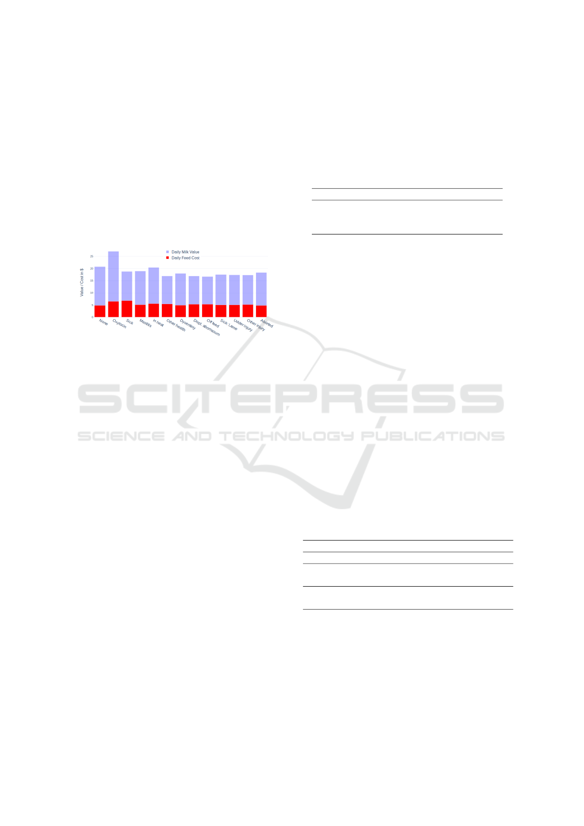
6.3 Health Data
We know that health and metabolic markers such as
SCC, MUN and BHB can help us predict the occur-
rence of diseases, hence drops in production. In fu-
ture research, it might be useful to collect full health
records and include them as input data since, we see
with the CAR codes that different types of condition
have different influences on the milk production (Fig-
ure 7). With the future acquisition of new veterinary
data we will be able to use them to develop a risk fac-
tor that could be used to improve the prediction of the
LSTM.
Figure 7: Disease Influence on the produced Milk Value
and the Feed costs.
6.4 Integrating other Data Type
Production data are not the only one available in the
dairy industry. Other types of data have been gathered
and could be used to fine tune our model.
6.4.1 Genetic Data
In the current state, our model is considering each se-
quence as an instance of the same cow. Using genetics
as a cow embedding would help our model to distin-
guish two cows and make more specific predictions.
Many cows are also genotyped for the most frequent
genetic variants. These data would need extensive
feature engineering in order to keep the input reason-
ably small, but some research has already been con-
ducted on this matter (Calus et al., 2018). We could
then use the same method to integrate the genotypic
information in the first hidden state.
6.4.2 Feed Information
A key aspect to the dairy production is the food in-
take of the cow. The only data we used on this mat-
ter is a global feed cost c
i,t
, estimated by the farmer.
We used it to model the profit p
i,t
but not as a feature
itself. Nevertheless, it would be possible to retrieve
fine-grained data on this matter and thus build a more
accurate model. For now we only had feed cost for
30% of the cows and had to impute the rest with a
rather brutal method (herd mean or global mean). We
compared the prediction made by MuMu on the cows
who had information on their feed cost versus the one
who did not.
Table 5: Feed Cost influence, n is the number of cows,
mean and σ are the mean and the standard deviation of the
RMSE of the two predictions group.
With Feed Cost Without Feed Cost
n 67 227 70 515
mean 7.83 8.91
σ 6.48 7.42
It appeared to be significantly better (t = −78.1, p <
10
−12
) when there was information on Feed Cost. So
it seems like there are still place for improvement in
this direction.
6.5 Transfer Learning to Other Breeds
Typical model in the dairy industry are suited for only
one breed. So we chose to follow this choice and
train our model for the Holstein cows that constituted
92.8% of our dataset. We could therefore train our
model for other breeds and customize for each breed
even if we have few instances of them. We asked
our model to predict the profit for the cows of other
species and it showed some interesting results. It
failed to outperform ARIMA for the CN breed be-
cause there production is quite different from the HO
breed and we have very few examples.
Table 6: Performance across breeds, Breeds: AY = Ayr-
shire, BS = Brown Swiss, CN = Canadienne, JE = Jersey,
n is the number of cows, RMSE and MAE are the errors in
dollar, over is the percentage the cows over-estimated in our
recommendation, under is the percentage of cows under-
estimated by our model.
AY JE BS CN
n 19 432 8 346 2 794 847
RMSE
MuMu
9.72 9.09 8.49 12.6
RMSE
ARIMA
13.5 12.9 13.3 10.8
MAE
MuMu
7.54 7.10 6.32 10.9
MAE
ARIM
10.4 9.71 9.90 8.30
7 CONCLUSION
This paper presents a first attempt to predict the fu-
ture profit of cows based on early information. The
proposed models achieves better results than ARIMA
statistical model. This shows that data-driven can be
ICAART 2020 - 12th International Conference on Agents and Artificial Intelligence
956

used to improve decisions made by farmers and in-
crease their profit. With such models, they can an-
ticipate almost any decision. Future direction is to
include more data and integrate new factors. We also
shed light on some interesting paths we should follow
in order to improve the results.
REFERENCES
Abadi, M., Barham, P., Chen, J., Chen, Z., Davis, A.,
Dean, J., Devin, M., Ghemawat, S., Irving, G., Isard,
M., et al. (2016). Tensorflow: A system for large-
scale machine learning. In 12th {USENIX} Sympo-
sium on Operating Systems Design and Implementa-
tion ({OSDI} 16), pages 265–283.
Auldist, M. and Hubble, I. (1998). Effects of mastitis on
raw milk and dairy products. Australian journal of
dairy technology, 53(1):28.
Bengio, Y., Simard, P., Frasconi, P., et al. (1994). Learning
long-term dependencies with gradient descent is diffi-
cult. IEEE transactions on neural networks, 5(2):157–
166.
Borchers, M., Chang, Y., Proudfoot, K., Wadsworth, B.,
Stone, A., and Bewley, J. (2017). Machine-learning-
based calving prediction from activity, lying, and ru-
minating behaviors in dairy cattle. Journal of dairy
science, 100(7):5664–5674.
Box, G. E., Jenkins, G. M., and Reinsel, G. (1970). Time se-
ries analysis: forecasting and control holden-day san
francisco. BoxTime Series Analysis: Forecasting and
Control Holden Day1970.
Box, G. E., Jenkins, G. M., Reinsel, G. C., and Ljung, G. M.
(2015). Time series analysis: forecasting and control.
John Wiley & Sons.
Bruinsma, J. (2017). World agriculture: towards
2015/2030: an FAO study. Routledge.
Calus, M., Goddard, M., Wientjes, Y., Bowman, P., and
Hayes, B. (2018). Multibreed genomic prediction us-
ing multitrait genomic residual maximum likelihood
and multitask bayesian variable selection. Journal of
dairy science, 101(5):4279–4294.
Canova, F. and Hansen, B. E. (1995). Are seasonal patterns
constant over time? a test for seasonal stability. Jour-
nal of Business & Economic Statistics, 13(3):237–
252.
Cho, K., Van Merri
¨
enboer, B., Gulcehre, C., Bahdanau, D.,
Bougares, F., Schwenk, H., and Bengio, Y. (2014).
Learning phrase representations using rnn encoder-
decoder for statistical machine translation. arXiv
preprint arXiv:1406.1078.
Choi, E., Bahadori, M. T., Schuetz, A., Stewart, W. F., and
Sun, J. (2016). Doctor ai: Predicting clinical events
via recurrent neural networks. In Machine Learning
for Healthcare Conference, pages 301–318.
Chollet, F. e. a. (2015). Keras. https://keras.io.
Contreras, J., Espinola, R., Nogales, F. J., and Conejo,
A. J. (2003). Arima models to predict next-day elec-
tricity prices. IEEE transactions on power systems,
18(3):1014–1020.
Dohoo, I. R. and Martin, S. (1984). Subclinical ketosis:
prevalence and associations with production and dis-
ease. Canadian Journal of Comparative Medicine,
48(1):1.
Emmons, D., Tulloch, D., and Ernstrom, C. (1990).
Product-yield pricing system. 1. technological consid-
erations in multiple-component pricing of milk. Jour-
nal of dairy science, 73(7):1712–1723.
Erdman, R. A. and Varner, M. (1995). Fixed yield responses
to increased milking frequency. Journal of dairy sci-
ence, 78(5):1199–1203.
Graves, A., Mohamed, A.-r., and Hinton, G. (2013).
Speech recognition with deep recurrent neural net-
works. In 2013 IEEE international conference on
acoustics, speech and signal processing, pages 6645–
6649. IEEE.
Graves, A. and Schmidhuber, J. (2009). Offline handwrit-
ing recognition with multidimensional recurrent neu-
ral networks. In Advances in neural information pro-
cessing systems, pages 545–552.
Grinblat, G. L., Uzal, L. C., Larese, M. G., and Granitto,
P. M. (2016). Deep learning for plant identification
using vein morphological patterns. Computers and
Electronics in Agriculture, 127:418–424.
Hochreiter, S. and Schmidhuber, J. (1997). Lstm can solve
hard long time lag problems. In Advances in neural
information processing systems, pages 473–479.
Hyndman, R. and Khandakar, Y. (2007). Automatic time
series forecasting: the forecast package for r 7, 2008.
URL http://www. jstatsoft. org/v27/i03.
Jones, J. W., Antle, J. M., Basso, B., Boote, K. J., Co-
nant, R. T., Foster, I., Godfray, H. C. J., Herrero, M.,
Howitt, R. E., Janssen, S., et al. (2017). Toward a
new generation of agricultural system data, models,
and knowledge products: State of agricultural systems
science. Agricultural systems, 155:269–288.
Kamilaris, A. and Prenafeta-Bold
´
u, F. X. (2018). Deep
learning in agriculture: A survey. Computers and elec-
tronics in agriculture, 147:70–90.
Kussul, N., Lavreniuk, M., Skakun, S., and Shelestov, A.
(2017). Deep learning classification of land cover and
crop types using remote sensing data. IEEE Geo-
science and Remote Sensing Letters, 14(5):778–782.
Kuwata, K. and Shibasaki, R. (2015). Estimating crop
yields with deep learning and remotely sensed data.
In 2015 IEEE International Geoscience and Remote
Sensing Symposium (IGARSS), pages 858–861. IEEE.
Kwiatkowski, D., Phillips, P. C., Schmidt, P., and Shin,
Y. (1992). Testing the null hypothesis of stationarity
against the alternative of a unit root: How sure are we
that economic time series have a unit root? Journal of
econometrics, 54(1-3):159–178.
Lipton, Z. C., Kale, D. C., Elkan, C., and Wetzel, R. (2015).
Learning to diagnose with lstm recurrent neural net-
works. arXiv preprint arXiv:1511.03677.
Maupom
´
e, D., Queudot, M., and Meurs, M.-J. (2019). In-
ter and intra document attention for depression risk
assessment. In Canadian Conference on Artificial In-
telligence, pages 333–341. Springer.
Nair, V. and Hinton, G. E. (2010). Rectified linear units
improve restricted boltzmann machines. In Proceed-
Towards an Effective Decision-making System based on Cow Profitability using Deep Learning
957

ings of the 27th international conference on machine
learning (ICML-10), pages 807–814.
Rahnemoonfar, M. and Sheppard, C. (2017). Deep count:
fruit counting based on deep simulated learning. Sen-
sors, 17(4):905.
Ray, D., Halbach, T., and Armstrong, D. (1992). Season and
lactation number effects on milk production and re-
production of dairy cattle in arizona. Journal of dairy
science, 75(11):2976–2983.
Rumelhart, D. E., Hinton, G. E., Williams, R. J., et al.
(1988). Learning representations by back-propagating
errors. Cognitive modeling, 5(3):1.
Schaeffer, L. and Jamrozik, J. (1996). Multiple-trait pre-
diction of lactation yields for dairy cows. Journal of
Dairy Science, 79(11):2044–2055.
Schmidhuber, J., Wierstra, D., and Gomez, F. J. (2005).
Evolino: Hybrid neuroevolution/optimal linear search
for sequence prediction. In Proceedings of the 19th In-
ternational Joint Conferenceon Artificial Intelligence
(IJCAI).
Sladojevic, S., Arsenovic, M., Anderla, A., Culibrk, D., and
Stefanovic, D. (2016). Deep neural networks based
recognition of plant diseases by leaf image classifi-
cation. Computational intelligence and neuroscience,
2016.
Smith, T. G. et al. (2017). pmdarima: Arima estimators for
Python. http://www.alkaline-ml.com/pmdarima.
Song, X., Zhang, G., Liu, F., Li, D., Zhao, Y., and Yang, J.
(2016). Modeling spatio-temporal distribution of soil
moisture by deep learning-based cellular automata
model. Journal of Arid Land, 8(5):734–748.
Ushikubo, S., Kubota, C., and Ohwada, H. (2017). The
early detection of subclinical ketosis in dairy cows
using machine learning methods. In Proceedings of
the 9th International Conference on Machine Learn-
ing and Computing, pages 38–42. ACM.
Wood, P. (1967). Algebraic model of the lactation curve in
cattle. Nature, 216(5111):164.
Zhang, G., Patuwo, B. E., and Hu, M. Y. (1998). Forecast-
ing with artificial neural networks:: The state of the
art. International journal of forecasting, 14(1):35–62.
Zhang, J., Zhu, Y., Zhang, X., Ye, M., and Yang, J. (2018).
Developing a long short-term memory (lstm) based
model for predicting water table depth in agricultural
areas. Journal of hydrology, 561:918–929.
ICAART 2020 - 12th International Conference on Agents and Artificial Intelligence
958
