A Novel Dispersion Covariance-guided One-Class Support Vector

Machines

Soumaya Nheri

, Riadh Ksantini

1,2

, Mohamed-B

echa Ka

aniche

and Adel Bouhoula

Higher School of Communication of Tunis, Research Lab: Digital Security, University of Carthage, Carthage, Tunisia

University of Windsor, 401, Sunset Avenue, Windsor, ON, Canada

Keywords:

Support Vector Machine, Kernel Covariance Matrix, One-Class Classiﬁcation, Outlier Detection, Low

Variances, Subclass Information.

Abstract:

In order to handle spherically distributed data, in a proper manner, we intend to exploit the subclass informa-

tion. In one class classiﬁcation process, many recently proposed methods try to incorporate subclass informa-

tion in the standard optimization problem. We presume that we should minimize the within-class variance,

instead of minimizing the global variance, with respect to subclass information. Covariance-guided One-Class

Support Vector Machine (COSVM) emphasizes the low variance direction of the training dataset which results

in higher accuracy. However, COSVM does not handle multi-modal target class data. More precisely, it does

not take advantage of target class subclass information. Therefore, to reduce the dispersion of the target data

with respect to newly obtained subclass information, we express the within class dispersion and we incorpo-

rate it in the optimization problem of the COSVM. So, we introduce a novel variant of the COSVM classiﬁer,

namely Dispersion COSVM, that exploits subclass information in the kernel space, in order to jointly mini-

mize the dispersion within and between subclasses and improve classiﬁcation performance. A comparison of

our method to contemporary one-class classiﬁers on numerous real data sets demonstrate clearly its superiority

in terms of classiﬁcation performance.

1 INTRODUCTION

The important motivation of one-class classiﬁcation

(OCC) has been studied under three main frame-

works. First, generally, it is assumed that information

from normal operation (targets) are easy to collect

during a training process, but most faults (outliers)

are not available or very costly to measure. For in-

stance, it is possible to measure the necessary features

for a nuclear power plant operating under normal cir-

cumstances. But, in case of accident, it is too dan-

gerous or impossible to measure the same features.

Second, outliers are badly represented and poorly dis-

tributed for training. This appears mainly in tumour

detection or rare medical diseases, where a limited

number of outliers are available during the training

process. Third, for many learning tasks, many ob-

jects are unlabeled and few labeled examples are al-

ways available, but they are badly represented with

unknown prior and ill-deﬁned distributions. For these

reasons, OCC problem can be found in many prac-

tical applications, such as, medical analysis (Gard-

ner et al., 2006), anomaly detection, face recognition

(Zeng et al., 2006) and web page classiﬁcation (Qi

and Davison, 2009).

In OCC problems, to classify future data points

as targets or outliers, three different categories of

OCC method can be used: density-based methods,

boundary-based methods and reconstruction-based

methods. Density-based methods, like Parzen density

estimator (Muto and Hamamoto, 2001) and Gaussian

distribution (Parra et al., 1996), are based on the es-

timation of the probability density function (PDF) of

the target class. In boundary-based classiﬁers, only

the boundary points around the target class are used to

classify data (Vapnik, 1998). The Support Vector Ma-

chine (SVM) (Cristianini and Shawe-Taylor, 2000) is

a popular two-class classiﬁcation method based on

this philosophy. It aims to maximize the distance mar-

gin between the two considered classes using support

vectors. It also found its application in OCC prob-

lem as One-Class SVM (OSVM) (Sch

olkopf et al.,

2001) and Support Vector Data Description (SVDD)

(Sadeghi and Hamidzadeh, 2018). Reconstruction-

based classiﬁers like k-means clustering (Ahmad and

Dey, 2011), have been introduced to model the data

546

Nheri, S., Ksantini, R., Kaâniche, M. and Bouhoula, A.

A Novel Dispersion Covariance-guided One-Class Support Vector Machines.

DOI: 10.5220/0009174205460553

In Proceedings of the 15th International Joint Conference on Computer Vision, Imaging and Computer Graphics Theory and Applications (VISIGRAPP 2020) - Volume 4: VISAPP, pages

546-553

ISBN: 978-989-758-402-2; ISSN: 2184-4321

rather than resolving classiﬁcation problem. During

classiﬁcation, a reconstruction error for the incoming

data point is calculated. The less the error, the more

accurate is the model. The main problems with these

three categories of one-class classiﬁcation methods

are that none of them consider the full scale of in-

formation available for classiﬁcation. For instance,

the density-based methods focus only on high den-

sity area and neglect areas with lower training data

density. In boundary-based methods, the solutions

are only calculated based on the points near the deci-

sion boundary, regardless the spread of the remaining

data. A more reasonable method would be to simul-

taneously make use of the maximum margin criterion

(Cristianini and Shawe-Taylor, 2000), while control-

ling the spread of data. Besides, unlike multi-class

classiﬁcation problems, the low variance directions

of the target class distribution are crucial for OCC.

In (Kwak and Oh, 2009), it has been shown that pro-

jecting the data in the high variance directions (like

PCA) will result in higher error (bias), while retain-

ing the low variance directions will lower the total

error. Boundary-based methods privilege separating

data along large variance directions and do not put

special emphasis on low variance directions (Shiv-

aswamy and Jebara, 2010). Moreover, we need to re-

duce the estimation error by taking projections along

some variance directions and the estimated covari-

ance is not accurate due to the limited number of train-

ing samples.

However, taking these projections before train-

ing leads to an important loss of characteristics.

Some powerful classiﬁers have been proposed to take

the overall structural information of the training set

into account through the incorporation of the co-

variance matrix into the objective OSVM function

then we can mention the most relevant among them:

The Mahalanobis One-class SVM (MOSVM) (Tsang

et al., 2006), the Relative Margin Machines (RMM)

(Shivaswamy and Jebara, 2010) and the Discrimi-

nant Analysis via Support Vectors(SVDA) (Gu et al.,

2010). In the one-class domain, the most relevant

work is the Covariance-guided One-class Support

Vector Machine (COSVM) (Khan et al., 2014). The

principal motivation behind COSVM method is to put

more emphasis on the low variance directions by in-

corporates the covariance matrix into object function

of the OSVM (Sch

olkopf et al., 2001). In fact, before

training, we want to keep all data characteristics and

use the maximum margin based solution, while taking

projections in speciﬁc directions. In terms of classi-

ﬁcation performance, COSVM was shown to be very

competitive with SVDD, OSVM and MOSVM.

However, there are still some difﬁculties asso-

ciated with COSVM application in real case prob-

lems, where data are highly dispersed and the tar-

get class can be divided into subclasses. In order to

handle spherically distributed data, in a proper man-

ner, we intend to exploit the subclass information. In

one class classiﬁcation process, many recently pro-

posed methods try to incorporate subclass informa-

tion in the standard optimization problem. We can

mention among them: The Subclass One-Class Sup-

port Vector machine (SOC-SVM) (Mygdalis et al.,

2015) and the Kernel Support Vector Description

(KSVDD) (Mygdalis et al., 2016). The basic prin-

ciple of the SOC-SVM method is to introduce a novel

variant of the OSVM classiﬁer that exploits subclass

information, in order to minimize the data disper-

sion within each subclass and determine the optimal

decision function. Experimental results denote that

(SOC-SVM) approach is able to outperform OSVM

in video segments selection. On the other hand,

KSVDD method modiﬁes the standard SVDD opti-

mization process and extends the proposed method

to work in feature spaces of arbitrary dimensional-

ity. Comparative results of KSVDD with the OSVM,

the standard SVDD and the minimum variance SVDD

(MV-SVDD)(Zafeiriou and Laskaris, 2008) demon-

strate the superiority of KSVDD. We presume that we

should minimize the within-class variance, instead of

minimizing the global variance, with respect to sub-

class information. Thus, a clustering step is achieved

in order to estimate the existing subclasses into the

target class. Furthermore, It has been shown in (Zhu

and Martinez, 2006) that the clustering does not have

a major impact in the classiﬁcation accuracy. Hence,

any clustering algorithm can work in this approach.

Then, to reduce the dispersion of the target data with

respect to newly obtained subclass information, we

express the within class dispersion and we incorpo-

rate it in the optimization problem of the COSVM.

In this paper, we propose a novel Dispersion

COSVM (DCOSVM), which incorporates a dis-

persion matrix into the objective function of the

COSVM, in order to reduce the dispersion of the tar-

get data with respect to newly obtained subclass in-

formation and improve classiﬁcation accuracy. Un-

like the SOC-SVM and the KSVDD methods, the

DCOSVM has the advantage of minimizing not only

the data dispersion within each subclass, but also data

dispersion between subclasses, in order to improve

classiﬁcation performance. Moreover, the DCOSVM

utilizes a trade off controlling parameter to ﬁne-tune

the effect of the dispersion matrix on the classiﬁca-

tion accuracy. The proposed method is still based on

a convex optimization problem, where a global op-

A Novel Dispersion Covariance-guided One-Class Support Vector Machines

547

timal solution could be estimated easily using exist-

ing numerical methods. The rest of the paper is orga-

nized as follows: The next section describes in details

a novel subclass method based on COSVM. Section

3 presents a comparative evaluation of our method to

other state of the art relevant one-class classiﬁers, on

several common datasets. Finally, Section 4 contains

some concluding remarks.

2 THE NOVEL DISPERSION

COSVM

In this section we describe in details our proposed

method. First, we present the COSVM method which

provides more importance towards the low variance

directions by incorporating the estimated covariance

matrix of target class.

2.1 The COSVM Method

The estimated covariance matrix of the training data

contains all projectional directions, from high vari-

ance to low variance. Thus, to keep the robustness

of the OSVM classiﬁer intact while emphasizing the

small variance directions, (Khan et al., 2014) incor-

porate the kernel covariance matrix into the objective

function of the OSVM optimization problem. So, us-

ing the kernel trick, the convex optimization problem

of COSVM method can be described as follows:

min

(ηQ + (1 − η)∆)α (1)

s.t. 0 ≤ α

≤

∑

i=1

= 1,

where

∆ = Q(I − 1

. (2)

For clarity, we have used the vectorized form of α =

(α

,.. .,α

) and v ∈ (0, 1] is the key parameter that

controls the fraction of outliers and that of support

vectors (SVs). Q is the kernel matrix as deﬁned in

Eq. (3):

Q(i, j) = K (x

), (3)

i = 1, ... ,N; j = 1, ... ,N.

I is the identity matrix and 1

is a matrix with all en-

tries

, and η is the tradeoff parameter that controls

the balance between the kernel matrix Q and the dual

kernel covariance matrix ∆. According to (Khan et al.,

2014), by controlling the value of v in the training

phase, one can control the conﬁdence on the training

dataset directly. If the training dataset is very reliable,

v can be set to a low value so that the whole training

dataset is considered. On the other hand, if it is not

known whether or not the training dataset truly rep-

resents the target class, v can be set to some higher

value.

2.2 Derivation of Dispersion COSVM

(DCOSVM)

The DCOSVM takes into account the subclass dis-

tribution in order to provide more efﬁcient and ro-

bust solutions than standard COSVM. The whole idea

is based onto projecting the training data set of N

samples, X = {x

}

i=1

to a higher dimensional fea-

ture space F = {Φ(x

)}

i=1

by the function Φ, where

linear classiﬁcation might be achieved. In practice,

F is not calculated directly. The kernel trick (Vap-

nik, 1998) is used to calculate the mapping, where

a kernel function K calculates the inner products of

the higher dimensional data samples: K (x

) =<

Φ(x

),Φ(x

) >,∀i, j ∈ {1, 2,.. ., N}. After mapping

to feature space, since the entire training set belongs

to one class only, we cluster all the training vec-

tors in order to determine K clusters {C

}

d=1

, where

| = N

,∀d ∈ {1, 2,.. .,K}. Let m

denotes the

mean of the cluster C

samples calculated in feature

space:

∑

i=1

Φ(x

). (4)

We used m

to calculate the kernel covariance matrix

of the training cluster C

∑

i=1

(Φ(x

) − m

)(Φ(x

) − m

)

. (5)

Considering the case where K subclasses are formed

within the target class, the within subclass scatter ma-

trix (dispersion of the training vectors) can be ex-

pressed as follows:

∑

d=1

(

). (6)

Where

is the prior probability of the d − th sub-

class. The between scatter matrix can be deﬁned as

follows:

∑

d=1

∑

b=1,b6=d

− m

)(m

− m

)

. (7)

Using this deﬁnition, we incorporate the within sub-

class and between subclass scatter matrices as an ad-

ditional w

w and w

w, respectively, into the

VISAPP 2020 - 15th International Conference on Computer Vision Theory and Applications

548

objective function of the optimization problem of

COSVM Eq. (1). In fact, the term w

w is used to

minimize the dispersion within subclasses, whereas

the term w

w has the advantage of minimizing

the dispersion between subclasses. However, the

dual problem is the one that is solved through some

optimization algorithm for COSVM, not the primal

one. Thus, it is more appropriate to incorporate the

subclass scatter matrix directly in the dual problem.

Therefore, we have to use the kernel trick to repre-

sent the additional term w

in terms of dot prod-

ucts only. From the theory of reproducing kernels, we

know that any solution w must lie in the span of all

training samples. Hence, we can ﬁnd an expansion of

w of the form:

w =

∑

i=1

Φ(x

). (8)

By using the deﬁnitions of Σ

Eq. (5), m

Eq. (4)

and the kernel function K (x

) =< Φ(x

),Φ(x

) >

,∀i, j ∈ {1,2,.. .,N}, we derive the dot product form

in Eq. (9), where Q is the kernel matrix as deﬁned in

Eq. (3). I is the identity matrix and 1

is a matrix

with all entries

∆

is the transformed version of Σ

to be used in the

dual form:

∆

= Q

(I − 1

. (10)

This form of kernel covariance matrix ∆

is only in

terms of the kernel function and can be calculated

easily using the kernel trick. Let M

is the “kernel

mean of cluster C

”, which is an N

dimensional vec-

tor. Each component of M

is deﬁned as:

)

∑

i=1

K (x

), ∀ j = 1,. .., N. (11)

Using this deﬁnition, the between scatter matrix S

deﬁned in Eq. (12).

Hence, our target term to incorporate into the

COSVM dual problem is:



∑

d=1

∆

∑

d=1

∑

b=1,b6=d

− M

)(M

− M

)



α.

(13)

With this replacement, our proposed Dispersion

COSVM method can be described by the optimiza-

tion problem deﬁned in Eq. (14).

w =



∑

i=1

)



∑

d=1

(

)



∑

k=1

Φ(x

)



(9)

∑

i=1

∑

k=1

∑

d=1

∑

j=1

)(Φ(x

) − m

)(Φ(x

) − m

)

Φ(x

)

∑

i=1

∑

k=1

∑

d=1

∑

j=1



K (x

) −

∑

l=1

K (x

)



K (x

) −

∑

m=1

K (x

)



∑

i=1

∑

k=1

∑

d=1

∑

j=1



K (x

)K (x

) −

2α

∑

l=1

K (x

)K (x

) +

∑

l=1

∑

m=1

K (x

)K (x

)



∑

i=1

∑

k=1

∑

d=1

∑

j=1



K (x

)K (x

) −

∑

l=1

K (x

)K (x

)



∑

d=1

− α

∑

d=1

(I − 1

= α

∑

d=1

∆

w =



∑

i=1

)



∑

d=1

∑

b=1,b6=d

− m

)(m

− m

)



∑

k=1

Φ(x

)



(12)

= α

∑

d=1

∑

b=1,b6=d

− M

)(M

− M

)

α.

A Novel Dispersion Covariance-guided One-Class Support Vector Machines

549

min

ηQα + α

(1 − η)



∑

d=1

∆

∑

d=1

∑

b=1,b6=d

− M

)(M

− M

)



α (14)

s.t. 0 ≤ α

≤

∑

i=1

= 1.

The proposed method still results in a convex op-

timization problem since both the kernel matrix Q

and the covariance matrix ∆ are positive deﬁnite

(Michelli, 1986; Horn and Charles, 1990). As a re-

sult, the solution to this optimization problem will

have one global optimum solution and can be solved

efﬁciently using numerical methods.

However, we control the balance between the disper-

sion matrix and the Kernel matrix through our control

parameter η.

2.3 The Impact of the Tradeoff

Parameter η

One important step for achieving better classiﬁcation

with DCOSVM is ﬁnding the appropriate value for η.

The contribution of our kernel matrix Q, the between

scatter matrix S

and the within subclass scatter ma-

trix S

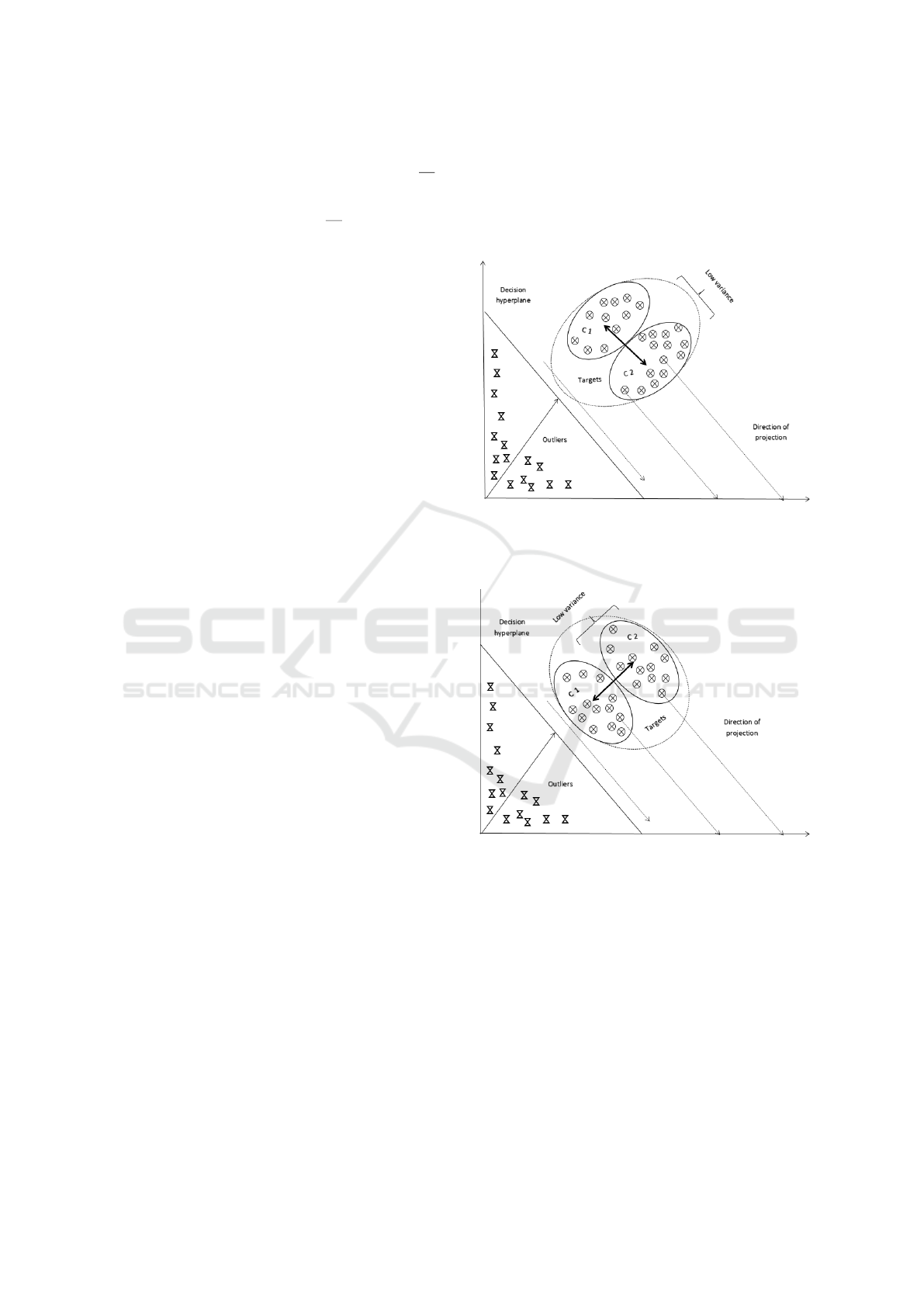
is controlled using the parameter η. Figure 1

shows the case where the optimal decision hyperplane

for the example target data is on the same direction

as the high variance. The control parameter η is set

equal to 1 which means the low variance directions

will not be given any special consideration in this

case. On the other hand, Figure 2 is the case when

the direction optimal of decision hyperplane and the

low variance are parallel. In this case, η can be set to

0. However, in real world cases (0 < η < 1), the op-

timal decision hyperplane is highly unlikely to be en-

tirely parallel to the direction of low variance or high

variance. For this reason, the value of η needs to be

tuned so that we have less overlap between the linear

projections of the target data and the outlier data. We

use an indirect approach to optimize η which will be

explained in detail in the next section.

2.4 Schematic Depictions

In this section, Figure 3 presents schematic depic-

tions to show the advantage of our DCOSVM method

over the unimodal COSVM.

3 EXPERIMENTAL RESULTS

This section presents the detailed experimental anal-

ysis and results for our proposed method, performed

on both artiﬁcial and benchmark real-world one-class

Figure 1: Case 1: Schematic depiction of the decision hy-

perplane for DCOSVM when the optimal linear projection

would be along the direction of high variance. In this case,

the optimal control parameter value for DCOSVM is η = 1.

Figure 2: Case 2: Schematic depiction of the decision hy-

perplane for DCOSVM when the optimal linear projection

would be along the direction of low variance. In this case,

the optimal control parameter value for DCOSVM is η = 0.

datasets, compared against contemporary one-class

classiﬁers.

3.1 Data Sets Used

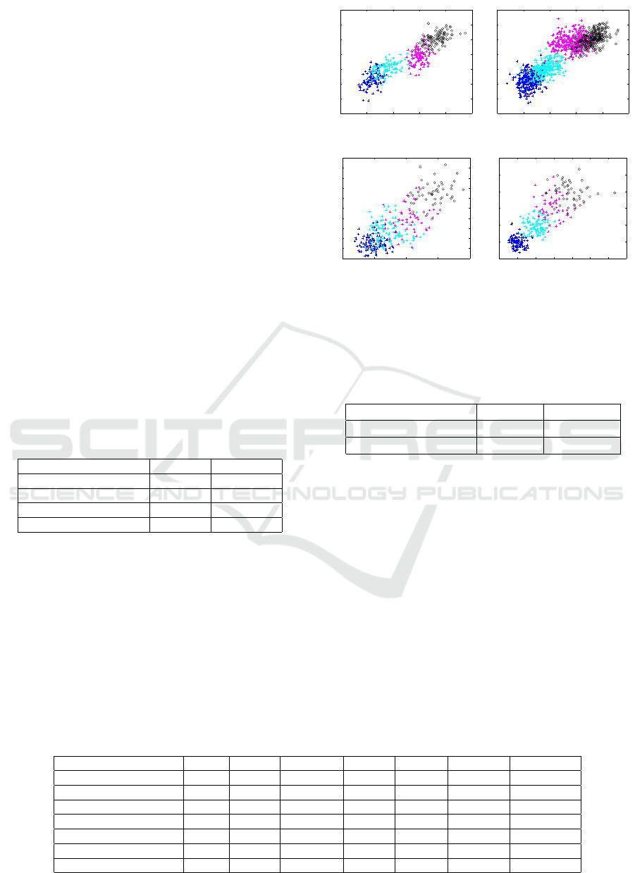
In our experiments, to test the robustness of our pro-

posed method in different scenarios, we have used

both artiﬁcially generated datasets and real world

datasets. For the experiments on artiﬁcially gener-

ated data, we have created several sets of 2D four-

class data drawn from two different sets of distribu-

VISAPP 2020 - 15th International Conference on Computer Vision Theory and Applications

550

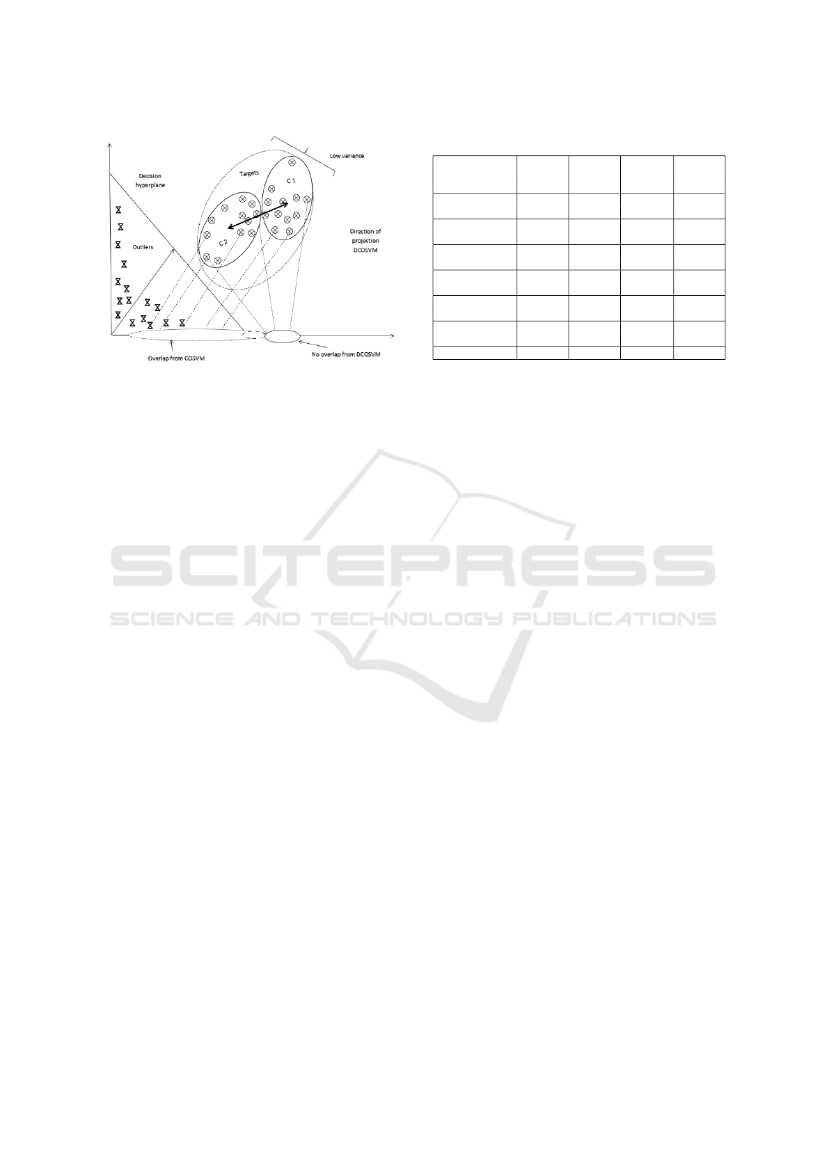
Figure 3: Comparison between COSVM and DCOSVM:

The value of the tradeoff parameter is set equal to 0 (η = 0),

to only consider the dispersion term.

tions: 1) Gaussian distributions with different covari-

ance matrices. 2) Gamma distributions with differ-

ent shape and scale parameters. For each distribution,

two different sets were created, one with low overlap

and the other with high overlap. Figure 4 shows the

plots of these generated data sets. We had a total 4

classes, one of the class is designated target and the

other ones as outlier. For the real world case, most of

these datasets were originally collected from the UCI

machine learning repository (Blake and Merz, 1999).

We have primarily focused on one of the important

ﬁelds of one-class classiﬁcation, such as, medical di-

agnosis (Fazli and Nadirkhanlou, 2013). Since these

datasets are originally multi- class, one of the class is

designated target and the other ones as outlier. Some

of the target and outlier sets were too trivial to clas-

sify. We have omitted those sets from our results. We

have also used varying size and dimensions of data

sets to test the robustness of our method against dif-

ferent feature sizes. As we can see from Table 1, the

dimensions vary from 3 to 300, while the training set

sizes vary from 21 to 288.

3.2 Experimental Protocol

The performance of the DCOSVM has been

compared to Covariance guided One-class SVM

(COSVM), One-class SVM (OSVM), Support Vec-

tor Data Description (SVDD), K Nearest Neighbors

(K-NN), Parzen, Gaussian. The classiﬁers are imple-

mented with the help of DDtools (Tax, 2012), and the

radial basis kernel was used for kernelization. This

kernel is calculated as K (x

) = e

−kx

−x

/σ

, where

σ represents the positive “width” parameter. For all

data sets used, we set the number of clusters C

min

= 2

and C

max

= 10 with the assumption that each data sets

Table 1: Description of Real Data Sets.

Data Number Number Number Number

set of of of of

Name Targets Outliers Features clusters

Haberman’s 81 225 3 2

Survival

Biomedical 67 127 5 4

(diseased)

Biomedical 127 67 5 4

(healthy)

SPECT Images 95 254 44 2

(normal)

Balance-scale 288 337 4 5

left

Balance-scale 288 337 4 4

right

waveform 21 600 300 3

target has a minimum of 2 clusters (sub-class) to a

maximum of 10 clusters. The number of subclasses is

determined by applying a clustering technique and the

validity index proposed in (Bouguessa et al., 2006),

on the samples belonging to each of the classes inde-

pendently. Second, we used 10-fold stratiﬁed cross

validation. In fact, we added 10% randomly selected

data to the outliers for testing, and the remaining was

used as the training data. To build different training

and testing sets, this approach was repeated 10 times.

The ﬁnal result was achieved by averaging over these

10 models. This ensures that the achieved results were

not a coincidence. Besides, to evaluate the methods,

we have used the Area Under the ROC Curve (AUC)

(Fawcett, 2006) produced by the ROC curves, and we

presented them in the results Table2. Consequently,

the AUC criterion must be maximized in order to ob-

tain a good separation between targets and outliers.

3.3 Results and Discussion

Table 2 and Table 4 contain the average AUC val-

ues obtained for the classiﬁers on the artiﬁcial and

real data sets. As we can see, the DCOSVM is su-

perior to all the other classiﬁers and provides best

results on almost data sets, in terms of the obtained

unbiased AUC values by averaging over 10 different

models. In fact, the DCOSVM has the advantage of

minimizing dispersion within and between subclasses

of the target class, thereby reducing overlapping and

improving classiﬁcation accuracy. In general, we see

that for real-world datasets (Table 4), the performance

of k-NN, Gaussian and Parzen classiﬁers are poor

when compared to the SVM-based classiﬁers (SVDD,

OSVM, COSVM). This is because of the limitations

inherent in these classiﬁers. Since k-NN classiﬁes a

data point solely based on its neighbors, it is sensi-

tive to outliers (Jiang and Zhou, 2004). The Gaussian

classiﬁer has some obvious limitations from the as-

A Novel Dispersion Covariance-guided One-Class Support Vector Machines

551

sumption that the underlying distribution is Gaussian,

which is not always the case for real datasets. The

Parzen classiﬁer is prone to degraded performance in

case of high-dimensional data or small sample size

(Muto and Hamamoto, 2001). We can easily see this

limitation of the Parzen classiﬁer from the poor re-

sults on the Gene Expression datasets which has a

very high dimension. The SVM-based classiﬁers are

free from all these assumptions and, hence, leads to

better result in majority of the cases. However, in case

of the artiﬁcial datasets (Table 2), we see that these

three classiﬁers (i.e. k-NN, Gaussian and Parzen) are

competitive with the SVM-based methods, sometimes

even better. This is because the artiﬁcial datasets are

generated from a pre-deﬁned regular distribution. We

see that the Gaussian method performs well for the

cases where the dataset was generated from a Gaus-

sian distribution, which is expected. It also performs

comparatively well for the datasets generated from the

banana distribution. This is because the banana dis-

tribution is actually generated by superimposing an

underlying Gaussian distribution on a banana shape.

However, in case of Gamma distribution, it performs

poorly since the distribution does not match with the

assumption of the classiﬁer.

Table 2: Average AUC of each method for the 4 artiﬁcial

data sets (best method in bold).

Dataset COSVM DCOSVM

Gauss. (low overlap) 95.66 96.88

Gauss. (high overlap) 88.29 91.10

Gamma (low overlap) 91.27 93.03

Gamma (high overlap) 98.17 98.69

In terms of training computational complexity,

the DCOSVM has almost the same complexity as

COSVM. In fact, the computation of dual kernel

covariance matrix can be done as part of the pre-

processing and re-used throughout the training phase.

The DCOSVM algorithm uses sequential minimal op-

timization to solve the quadratic programming prob-

lem, and therefore scales with is O(N

), where N is

the number of training data points (Sch

olkopf et al.,

2001). Table 3 shows the average training times for

both the artiﬁcial and the real-world datasets. As we

−5 0 5 10 15 20

−5

−5 0 5 10 15 20

−5

(a) Gaussian (low overlap) (b) Gaussian (high overlap)

0 50 100 150 200

100

120

140

160

180

200

220

0 50 100 150 200 250 300 350

100

150

200

250

300

Figure 4: Four artiﬁcial four-class datasets used for com-

parison. The blue class represents the target class (in each

subﬁgure caption).

Table 3: Average training times in milliseconds for COSVM

and DCOSVM for the experiments on the artiﬁcial and real-

world datasets.

Experiment COSVM DCOSVM

Artiﬁcial Datasets 7.4 8.5

Real-world Datasets 127.7 131.2

expect, DCOSVM has almost the same training time

as COSVM.

4 CONCLUSIONS

In this paper, we have improved COSVM classiﬁca-

tion approach by taking advantage of target class sub-

class information.The novel variant of the COSVM

classiﬁer, namely, Dispersion COSVM (DCOSVM),

minimizes the dispersion within and between sub-

classes and improves classiﬁcation performance. We

have compared our method against contemporary

one-class classiﬁers on several artiﬁcial and real-

world benchmark datasets. The results show the su-

Table 4: Average AUC of each method for the 7 real-world data sets (best method in bold, second best emphasized).

Dataset k-NN Parzen Gaussian SVDD OSVM COSVM DCOSVM

Biomedical (healthy) 36.83 40.02 64.66 81.38 82.65 85.80 89.81

Biomedical (diseased) 89.42 90.09 89.60 90.28 91.04 91.04 92.16

SPECT (normal) 84.28 96.45 93.90 92.32 95.29 96.79 97.81

Balance-scale left 87.78 91.23 92.09 94.20 96.13 97.19 98.51

Balance-scale right 87.76 91.23 91.95 94.72 97.57 97.69 98.82

Haberman’s Survival 66.49 67.97 60.09 68.87 69.62 69.59 70.28

waveform 87.78 97.02 92.10 97.20 97.19 97.23 98.36

VISAPP 2020 - 15th International Conference on Computer Vision Theory and Applications

552

periority of DCOSVM which provides signiﬁcantly

improved performance over the other classiﬁers. In

future work, we will validate the proposed DCOSVM

on security applications, such as, face recognition,

anomaly detection, etc.

REFERENCES

Ahmad, A. and Dey, L. (2011). A k-means type clustering

algorithm for subspace clustering of mixed numeric

and categorical datasets. Pattern Recognition Letters,

32(7):1062–1069.

Blake, C. and Merz, C. (1999). UCI repos-

itory of machine learning data sets.

http://www.ics.uci.edu/∼mlearn/MLRepository.html.

Bouguessa, M., Wang, S., and Sun, H. (2006). An objective

approach to cluster validation. Pattern Recognition

Letters, 27(13):1419–1430.

Cristianini, N. and Shawe-Taylor, J. (2000). An Introduction

to Support Vector Machines and Other Kernel-based

Learning Methods. Cambridge University Press, 1

edition.

Fawcett, T. (2006). An introduction to ROC analysis. Pat-

tern Recognition Letters, 27(8):861–874.

Fazli, S. and Nadirkhanlou, P. (2013). A novel method

for automatic segmentation of brain tumors in mri im-

ages. CoRR, abs/1312.7573.

Gardner, A. B., Krieger, A. M., Vachtsevanos, G. J., and

Litt, B. (2006). One-class novelty detection for seizure

analysis from intracranial eeg. Journal of Machine

Learning Research, 7:1025–1044.

Gu, S., Tan, Y., and He, X. (2010). Discriminant anal-

ysis via support vectors. Neurocomputing, 73(10-

12):1669–1675.

Horn, R. and Charles, R. (1990). Matrix Analysis. Cam-

bridge University Press.

Jiang, Y. and Zhou, Z.-H. (2004). Editing Training Data for

k-NN Classiﬁers with Neural Network Ensemble. In

International Symposium on Neural Networks, pages

356–361. IEEE Press.

Khan, N. M., Ksantini, R., Ahmad, I. S., and Guan, L.

(2014). Covariance-guided one-class support vector

machine. Pattern Recognition, 47(6):2165–2177.

Kwak, N. and Oh, J. (2009). Feature extraction for one-

class classiﬁcation problems: Enhancements to biased

discriminant analysis. Pattern Recognition, 42(1):17–

26.

Michelli, C. (1986). Interpolation of Scattered Data: Dis-

tance Matrices and Conditionally Positive Deﬁnite

Functions. Constructive Approximation, 2:11–22.

Muto, Y. and Hamamoto, Y. (2001). Improvement of the

Parzen classiﬁer in small training sample size situa-

tions. Intelligent Data Analysis, 5(6):477–490.

Mygdalis, V., Iosiﬁdis, A., Tefas, A., and Pitas, I. (2015).

Exploiting subclass information in one-class support

vector machine for video summarization. In ICASSP,

pages 2259–2263. IEEE.

Mygdalis, V., Iosiﬁdis, A., Tefas, A., and Pitas, I. (2016).

Kernel subclass support vector description for face

and human action recognition. In SPLINE, pages 1–5.

IEEE.

Parra, L., Deco, G., and Miesbach, S. (1996). Statisti-

cal independence and novelty detection with informa-

tion preserving nonlinear maps. Neural Computation,

8:260–269.

Qi, X. and Davison, B. D. (2009). Web page classiﬁca-

tion: Features and algorithms. ACM Comput. Surv.,

41(2):12:1–12:31.

Sadeghi, R. and Hamidzadeh, J. (2018). Automatic support

vector data description. Soft Comput., 22(1):147–158.

Sch

olkopf, B., Platt, J. C., Shawe-Taylor, J., Smola, A. J.,

and Williamson, R. C. (2001). Estimating the support

of a high-dimensional distribution. Neural Computa-

tion, 13(7).

Shivaswamy, P. K. and Jebara, T. (2010). Maximum relative

margin and data-dependent regularization. Journal of

Machine Learning Research, 11:747–788.

Tax, D. (2012). DDtools, the Data Description Toolbox for

Matlab. version 1.9.1.

Tsang, I. W., Kwok, J. T., and Li, S. (2006). Learning the

kernel in mahalanobis one-class support vector ma-

chines. In IJCNN, pages 1169–1175. IEEE.

Vapnik, V. N. (1998). Statistical Learning Theory. Wiley,

New York, NY, USA.

Zafeiriou, S. and Laskaris, N. A. (2008). On the improve-

ment of support vector techniques for clustering by

means of whitening transform. IEEE Signal Process.

Lett., 15:198–201.

Zeng, Z., Fu, Y., Roisman, G. I., Wen, Z., Hu, Y., and

Huang, T. S. (2006). Spontaneous emotional facial

expression detection. Journal of Multimedia, 1(5):1–

Zhu, M. and Martinez, A. M. (2006). Subclass discrimi-

nant analysis. IEEE Trans. Pattern Anal. Mach. Intell.,

28(8):1274–1286.

A Novel Dispersion Covariance-guided One-Class Support Vector Machines

553