
Optical Flow Estimation using a Correlation Image Sensor
based on FlowNet-based Neural Network
Toru Kurihara
a
and Jun Yu
Kochi University of Technology, 185 Miyanokuchi, Tosayamada-cho, Kami city, Kochi, Japan
Keywords:
Optical Flow, Correlation Image Sensor, Deep Neural Network, FlowNet.
Abstract:
Optical flow estimation is one of a challenging task in computer vision fields. In this paper, we aim to combine
correlation image that enables single frame optical flow estimation with deep neural networks. Correlation
image sensor captures temporal correlation between incident light intensity and reference signals, that can
record intensity variation caused by object motion effectively. We developed FlowNetS-based neural networks
for correlation image input. Our experimental results demonstrate proposed neural networks has succeeded in
estimating the optical flow.
1 INTRODUCTION
Optical flow is the two-dimensional velocity field that
describes the apparent motion of image patterns. It
has large applications such as detection and track-
ing of an object, separation from a background or
more generally segmentation, three-dimensional mo-
tion computation, etc. One of the most established
algorithms for optical flow determination is based on
the optical flow constraint (OFC) equation describing
the intensity-invariance of moving patterns with reg-
ularization term(Horn and Schunck, 1981).
These days a deep neural network methods with
convolutional neural networks(CNNs) are applied to
estimate optical flow (Weinzaepfel et al., 2013).
FlowNet(Dosovitskiy et al., 2015) is one of the suc-
cessful neural network for optical flow estimation.
They adopted FCN-like structure without Fully Con-
nected layers so that their method didn’t depends on
the input image size. They also proposed good refine-
ment structure, they successfully estimated fine flow
fields.
Ando et. al. applied correlation image sen-
sor(Ando and Kimachi, 2003) and weighted integral
method(Ando and Nara, 2009) to optical flow estima-
tion(Ando et al., 2009). They started from optical
flow partial differential equation(Horn and Schunck,
1981) and formulated exposure time in integral form
and developed a sensing system that detects velocity
vector distribution on an optical image with a pixel-
a
https://orcid.org/0000-0001-8347-0283
wise spatial resolution and a frame-wise temporal res-
olution. Kurihara et. al. implemented fast optical
flow estimation algorithm achieving 3ms for 640x512
pixel resolution, and 7.5ms for 1280x1024 pixel reso-
lution using GPU(Kurihara and Ando, 2013). They
also applied total variation minimization technique
for direct algebraic method of optical flow detection
using correlation image sensor(Kurihara and Ando,
2014).
In this paper, we propose to combine correlation
image that enables single frame optical flow estima-
tion and deep neural networks. In the following sec-
tion, we review the correlation image sensor, and
show proposed FlowNetS-based neural network for
correlation images. Then we showed experimental re-
sults.
2 PRINCIPLE
2.1 Correlation Image Sensor
The three-phase correlation image sensor (3PCIS) is
the two dimensional imaging device, which outputs
a time averaged intensity image g
0
(x,y) and a corre-
lation image g
ω
(x,y). The correlation image is the
pixel wise temporal correlation over one frame time
between the incident light intensity and three external
electronic reference signals.
The photo of the 640 × 512 three-phase correla-
tion image sensor is shown in Figure 1, and its pixel
Kurihara, T. and Yu, J.
Optical Flow Estimation using a Correlation Image Sensor based on FlowNet-based Neural Network.
DOI: 10.5220/0009172708470852
In Proceedings of the 15th International Joint Conference on Computer Vision, Imaging and Computer Graphics Theory and Applications (VISIGRAPP 2020) - Volume 4: VISAPP, pages
847-852
ISBN: 978-989-758-402-2; ISSN: 2184-4321
Copyright
c
2022 by SCITEPRESS – Science and Technology Publications, Lda. All rights reserved
847
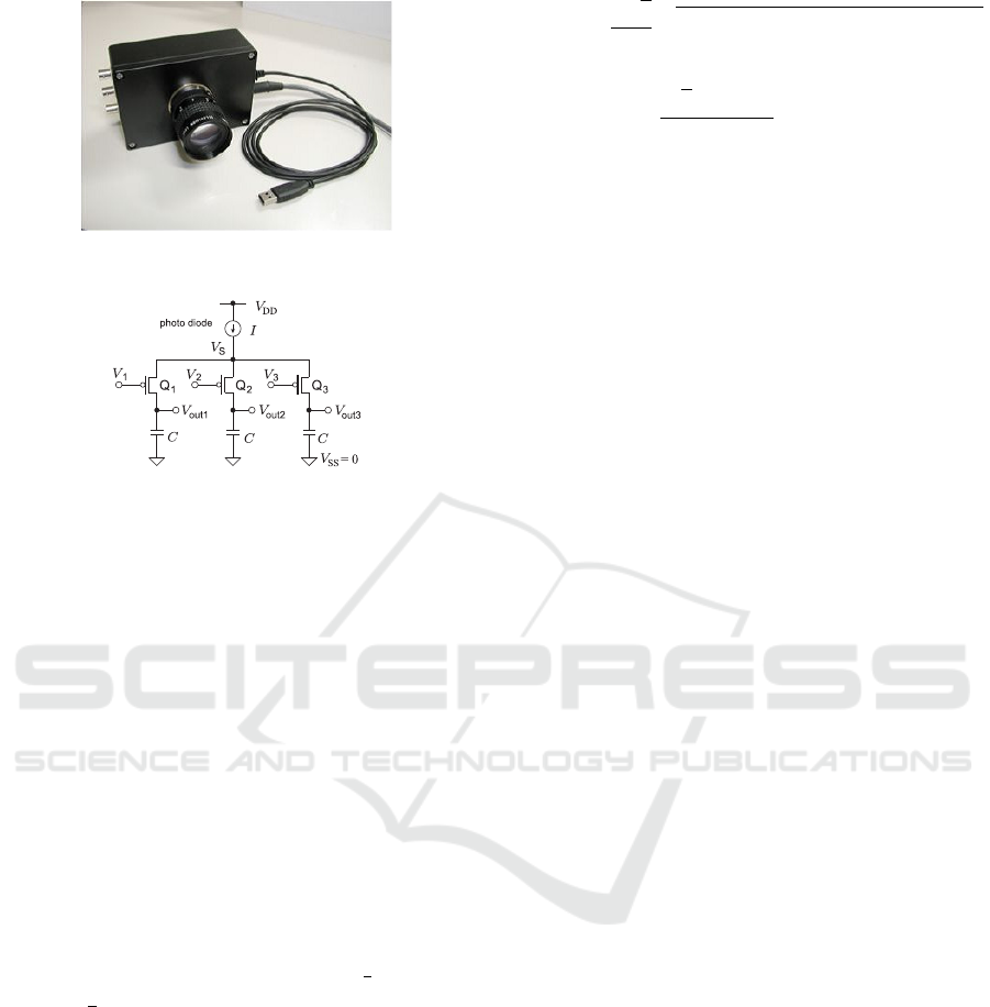
Figure 1: Photograph of Correlation Image Sensor(CIS).
Figure 2: Pixel structure of the correlation image sensor.
structure is shown in Figure 2.
Let T be frame interval and f (x,y,t) be instant
brightness of the scene, we have intensity image
g
0
(x,y) as
g
0
(x,y) =
Z
T
0
f (x,y,t) dt (1)
Let the three reference signals be v
k
(t) (k = 1,2,3)
where v
1
(t) + v
2
(t) + v
3
(t) = 0, the resulting correla-
tion image is written like this equation.
c
k
(x,y) =
Z
T
0
f (x,y,t) v
k
(t)dt (2)
Here we have three reference signals with one con-
straint, so that there remains 2 DOF for the basis of
the reference signal. We usually choose orthogonal si-
nusoidal wave pair (cosωt,sin ωt) as the basis, which
means v
1
(t) = cos ωt, v
2
(t) = cos(ωt +
2
3
π),v
3
(t) =
cos(ωt +
4
3
π).
Let the time-varying intensity in each pixel be
I(x, y,t) = A(x, y) cos(ωt + φ(x,y)) + B(x,y,t). (3)
Here A(x,y) and φ(x,y) is the amplitude and phase
of the frequency component ω, and B(x, y,t) is the
other frequency component of the intensity including
DC component. Due to the orthogonality, B(x,y,t)
doesn’t contribute in the outputs c
1
,c
2
,c
3
. Therefore
the amplitude and the phase of the frequency ω com-
ponent can be calculated as follows (Ando and Ki-
machi, 2003)
A(x,y) =
2
√
3
3
q
(c
1
−c
2
)
2
+ (c
2
−c
3
)
2
+ (c
3
−c
1
)
2
(4)
φ(x,y) = tan
−1
√
3(c
2
−c
3
)
2c
1
−c
2
−c
3
(5)
From the two basis of the reference signal
(cosnω
0
t,sin nω
0
t), we can rewrite amplitude and
phase using complex equation.
g
ω
(x,y) =
Z
T
0
f (x,y,t)e
−jωt
dt (6)
Here ω = 2πn/T . g
ω
(x,y) is the complex form of the
correlation image, and it is a temporal Fourier coeffi-
cient of the periodic input light intensity.
2.2 FlowNet-based Neural Network
We modified FlowNetSimple (Dosovitskiy et al.,
2015) for our purpose. The FlowNetSimple requires
two color images as input so that it has 6 channels
in the input layer. We change number of input chan-
nels in the input layer from 6 to 2. It means 2 chan-
nels for real part and imaginary part of the complex
correlation image. According to this reduction of the
input channels, we reduce the channels in latter lay-
ers, although we didn’t changed the other parameters
like kernel size, stride, and activation function. The
overall structure is shown in Fig.3. It has nine con-
volutional layers with stride of 2 and used ReLU ac-
tivation function after each layer. Convolutional fil-
ter sizes decrease towards deeper layers of networks:
7 ×7 for the first layer, 5 ×5 for the following two
layers and 3 ×3 for the rest of the layers. The number
of feature maps increases in the deeper layers.
We do not have any fully connected layers, which
allows the networks to take images of arbitrary size
as input. As training loss we use the endpoint er-
ror(EPE), which is used as standard error to measure
optical flow estimation. It is the average of Euclidean
distance of all pixels between the predicted flow and
the ground truth.
Using the same neural network structure, we com-
pared the proposed method with our modified gray
scale FlowNetS whose input is two still grayscale im-
ages.
3 EXPERIMENTS
3.1 Dataset
To evaluate our proposed method, we used computer
generated correlation images. In this simulation, we
VISAPP 2020 - 15th International Conference on Computer Vision Theory and Applications
848
conv1
conv2
conv3
conv3_1
conv4_1conv4
conv5
conv5_1
conv6
2 16
32
64
64 128
128
128
128
256
prediction
refinement
(a)
(b)
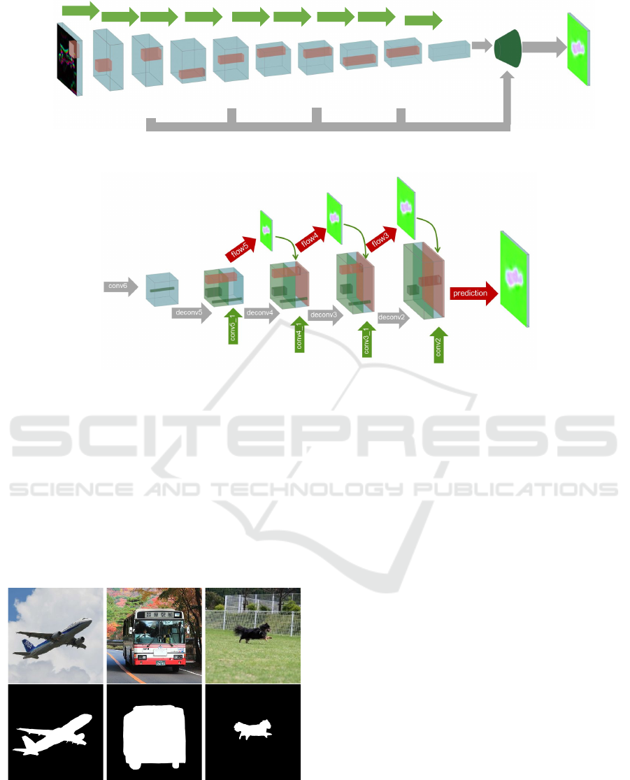
Figure 3: Proposed FlowNetS-based Network structure. The number of channels in input layer is reduced from 6 to 2 to
receive the correlation image. According to this reduction of the input channels, we reduce the channels in latter layers. Basic
structure follows FlowNetS structure. Each scale features are gathered in refinement block. (a)Overal structure, (b) refinement
block structure.
overlayed two images. Each image was moved uni-
formly in a random direction at random speed, in
other words each images moved at speed (v
x
,v
y
). In
addition, the upper image was used with mask of al-
pha channel. Those masks were generated by using
Photoshop manually. Examples of the still image are
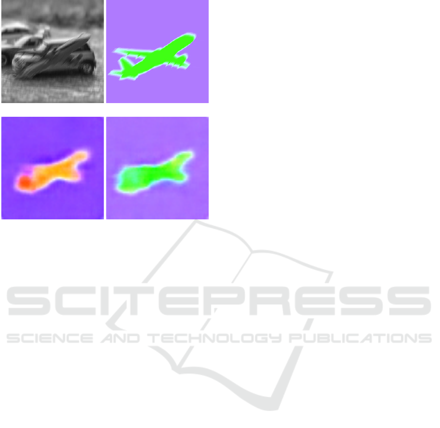
shown in Fig.4.
Figure 4: Examples of the still images and masks used for
simulation.
For the simulation, we divided one frame pe-
riod T into K samples with sampling duration ∆,
namely, T = K∆. The still image f (x, y) were shifted
(v
x
∆,v
y
∆) at each time-step when we assumed uni-
form motion. Then we can calculate intensity image
as follows,
g
0
(x,y) =
K−1
∑
k=0
f (x −v
x
k∆, y −v
y
k∆). (7)
And the correlation image is obtained as follows,
g
ω
0
(x,y) =
K−1
∑
k=0
f (x −v
x
k∆, y −v
y
k∆) exp(−jω
0
k∆).
(8)
Here we overlayed two images, f
f
(x,y) as fore-
ground and f
b
(x,y) as background, so that f (x,y) is
obtained by using foreground mask m
f
(x,y) as fol-
lows.
f (x,y) = f
f
(x,y)m
f
(x,y) + f
b
(x,y)(1 −m
f
(x,y))
(9)
The shifted image f (x −∆
x
,y −∆
y
) is obtained by us-
ing Fourier transform as follows.
f (x −∆
x
,y −∆
y
) = F
−1
[exp( ju∆
x
)exp( jv∆
y
)F(u,v)]
(10)
Here Fourier transform of f (x,y) is F(u,v) =
F [ f (x,y)], and u,v are spatial frequencies.
Optical Flow Estimation using a Correlation Image Sensor based on FlowNet-based Neural Network
849
We selected two images from 7 still images ran-
domly, and moved each images toward different di-
rection by using uniform random numbers, and gen-
erated 4096 sets of intensity image, correlation image
and two instant images. The 3276 sets were used for
training and the rest 820 sets were used for testing.
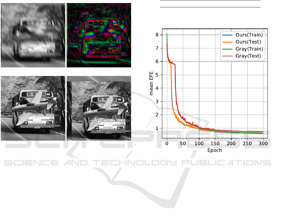
Figure (5) shows those calculated images.
(a) (b)
(c) (d)
Figure 5: Examples of the simulated images: (a) inten-
sity image, (b) correlation image, In addition, we used in-
stant images to compare the results: (c) instant image at
starting time,(k = 0 in eq.(7)) (d) instant image at end-
ing time(k = K −1 in eq.(7)) . In this simulation, fore-
ground image (airplane) moves (-8.25, -3.98) pixels and
background image (bus) moves (-7.93, -6.28) pixels during
exposure time.
3.2 Training Details
We adopted adam with a learning rate 0.0001 for opti-
mization. We used 300 epochs for training and batch
size was set to 8 for 3276 training data. We didn’t use
data augmentation technique in the experiments. We
implemented our models by the PyTorch framework
and trained them using a NVIDIA TITAN Xp GPU.
3.3 Results
To demonstrate effect of proposed method, we com-
pared proposed method to FlowNetS-based method.
In fact, two compared neural networks have the per-
fectly the same structure, but input images are differ-
ent. Proposed method has two input image of real part
of correlation image and imaginary part of correlation
image, compared method has also has two input im-
ages of still images of starting time and ending time.
The minimum EPE for testing data and training
are shown in Table 1. The minimum EPE of the pro-
posed method is better than the grayscale FlowNetS.
Table 1: Minimum end poinet error(EPE) over all epoch.
train test
Grayscale FlowNetS 0.635 0.727
Proposed 0.601 0.628
Figure 6: The results of training. (a) Mean end point error
(EPE) for training and testing of proposed method and gray
method”.
The results images are shown in Fig. 7, Fig.8,
Fig.9 and Fig.10. As illustrated in the Fig.7, both
the proposed method and the compared method looks
similar and shows good estimation results compared
to the ground truth. Figure 8 shows the best EPE re-
sults for both proposed and compared method. The
proposed method shows better estimation of the back-
ground motion. We consider that the large back-
ground area resulted in better EPE, since the second
best EPE has also dog foreground. Figure 9 shows
the worst EPE results for the proposed method. The
wings of the airplane is incomplete in the both meth-
ods. Figure 10 shows the worst EPE results for the
compared method. Although the velocity estimation
of the body of the airplane is wrong for compared
method, the proposed method shows better results.
The input images for the grayscale FlowNetS is
ideal instant one, which means we didn’t consider the
effect of motion blur. The faster the motion becomes,
more blur will occurs. This phenomenon makes it dif-
ficult to find correspondence between the two images.
We will investigate this further.
VISAPP 2020 - 15th International Conference on Computer Vision Theory and Applications
850
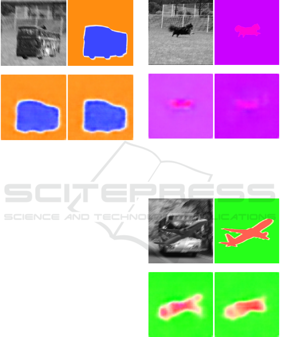
(a) (b)
(c) (d)
Figure 7: Examples of the estimated flow. foreground im-
age (bus) moves (-6.23, -9.10) pixels and background im-
age (dog) moves (-7.93, -6.28) pixels during exposure time:
(a) intensity image, (b) ground truth, (c) estimated by using
two instant images pair, (d) estimated by using correlation
image (proposed).
4 CONCLUSIONS
We proposed optical flow estimation method using a
deep neural network for correlation image. As the in-
put, the complex-valued correlation image is divided
in two channels, real value image and imaginary value
image. The proposed method enables single-frame
optical flow estimation. Right now, the accuracy of
the proposed method is similar to the conventional
one when we use the same neural network structure.
We point out that input images of grayscale FlowNetS
are the ideal one, which means there is no motion blur.
We need a further investigation about advantages of
the proposed method.
ACKNOWLEDGEMENTS
This work was supported by CASIO science promo-
tion foundation.
(a) (b)
(c) (d)
Figure 8: Best mean EPE examples of the estimated flow.
(Proposed:0.1596, Gray:0.1902) foreground image (dog)
moves (4.47, -2.35) pixels and background image (dog)
moves (3.23, -3.96) pixels during exposure time: (a) inten-
sity image, (b) ground truth, (c) estimated by using two in-
stant images pair, (d) estimated by using correlation image
(proposed).
(a) (b)
(c) (d)
Figure 9: Worst mean EPE examples for the proposed
method. (Proposed:1.652, Gray:1.687) foreground image
(airplane) moves (9.74, 1.49) pixels and background image
(dog) moves (-9.63, 8.74) pixels during exposure time: (a)
intensity image, (b) ground truth, (c) estimated by using two
instant images pair, (d) estimated by using correlation im-
age (proposed).
Optical Flow Estimation using a Correlation Image Sensor based on FlowNet-based Neural Network
851
(a) (b)
(c) (d)
Figure 10: Worst mean EPE examples for the grayscale
method. (Proposed:1.370, Gray:2.832) foreground image
(airplane) moves (-10.33, 11.25) pixels and background im-
age (car) moves (0.79, -8.56) pixels during exposure time:
(a) intensity image, (b) ground truth, (c) estimated by using
two instant images pair, (d) estimated by using correlation
image (proposed).
REFERENCES
Ando, S. and Kimachi, A. (2003). Correlation image sen-
sor: two-dimensional matched detection of amplitude-
modulated light. IEEE Transactions on Electron De-
vices, 50(10):2059–2066.
Ando, S., Kurihara, T., and Wei, D. (2009). Exact algebraic
method of optical flow detection via modulated inte-
gral imaging –theoretical formulation and real-time
implementation using correlation image sensor–. In
Proc. Int. Conf. Computer Vision Theory and Applica-
tions (VISAPP 2009), pages 480–487.
Ando, S. and Nara, T. (2009). An exact direct method
of sinusoidal parameter estimation derived from finite
fourier integral of differential equation. IEEE Trans-
actions on Signal Processing, 57(9):3317–3329.
Dosovitskiy, A., Fischer, P., Ilg, E., H
¨
ausser, P., Hazir-
bas, C., Golkov, V., v. d. Smagt, P., Cremers, D., and
Brox, T. (2015). Flownet: Learning optical flow with
convolutional networks. In 2015 IEEE International
Conference on Computer Vision (ICCV), pages 2758–
2766.
Horn, B. K. and Schunck, B. G. (1981). Determining optical
flow. Artificial Intelligence, 17(1):185 – 203.
Kurihara, T. and Ando, S. (2013). Fast optical flow detec-
tion based on weighted integral method using corre-
lation image sensor and gpu(in japanese). volume 3,
pages 170–171.
Kurihara, T. and Ando, S. (2014). Tv minimization of direct
algebraic method of optical flow detection via modu-
lated integral imaging using correlation image sensor.
In 2014 International Conference on Computer Vision
Theory and Applications (VISAPP), volume 3, pages
705–710.
Weinzaepfel, P., Revaud, J., Harchaoui, Z., and Schmid, C.
(2013). Deepflow: Large displacement optical flow
with deep matching. In The IEEE International Con-
ference on Computer Vision (ICCV).
VISAPP 2020 - 15th International Conference on Computer Vision Theory and Applications
852
