Two-step Multi-spectral Registration Via Key-point Detector and

Gradient Similarity: Application to Agronomic Scenes for Proxy-sensing

Jehan-Antoine Vayssade

, Gawain Jones

, Jean-Noel Paoli

and Christelle Gee

Agro

ecologie, AgroSup Dijon, INRA, Univ. Bourgogne-Franche-Comt

e, F-21000 Dijon, France

Keywords:

Registration, Multi-spectral Imagery, Precision Farming, Feature Descriptor.

Abstract:

The potential of multi-spectral images is growing rapidly in precision agriculture, and is currently based on the

use of multi-sensor cameras. However, their development usually concerns aerial applications and their pa-

rameters are optimized for high altitudes acquisition by drone (UAV ≈ 50 meters) to ensure surface coverage

and reduce technical problems. With the recent emergence of terrestrial robots (UGV), their use is diverted

for nearby agronomic applications. Making it possible to explore new agronomic applications, maximizing

speciﬁc traits extraction (spectral index, shape, texture . . . ) which requires high spatial resolution. The prob-

lem with these cameras is that all sensors are not aligned and the manufacturers’ methods are not suitable for

close-ﬁeld acquisition, resulting in offsets between spectral images and degrading the quality of extractable

informations. We therefore need a solution to accurately align images in such condition.

In this study we propose a two-steps method applied to the six-bands Airphen multi-sensor camera with (i)

afﬁne correction using pre-calibrated matrix at different heights, the closest transformation can be selected via

internal GPS and (ii) perspective correction to reﬁne the previous one, using key-points matching between en-

hanced gradients of each spectral bands. Nine types of key-point detection algorithms (ORB, GFTT, AGAST,

FAST, AKAZE, KAZE, BRISK, SURF, MSER) with three different modalities of parameters were evaluated

on their speed and performances, we also deﬁned the best reference spectra on each of them. The results show

that GFTT is the most suitable methods for key-point extraction using our enhanced gradients, and the best

spectral reference was identiﬁed to be the band centered on 570 nm for this one. Without any treatment the

initial error is about 62 px, with our method, the remaining residual error is less than 1 px, where the man-

ufacturer’s involves distortions and loss of information with an estimated residual error of approximately 12

px.

1 INTRODUCTION

Modern agriculture is changing towards a system that

is less dependent on pesticides (Lechenet et al., 2014)

(herbicides remain the most difﬁcult pesticides to re-

duce) and digital tools are of great help in his mat-

ter. The development of imaging and image process-

ing have made it possible to characterize an agricul-

tural plot (Sankaran et al., 2015) (crop health sta-

tus or soil characteristics) using non-destructive agro-

nomic indices (Jin et al., 2013) replacing traditional

destructive and time-consuming methods. In recent

years, the arrival of miniaturized multi-spectral and

hyper-spectral cameras on Unmanned Aerial Vehicles

https://orcid.org/0000-0002-7418-8347

https://orcid.org/0000-0002-5492-9590

https://orcid.org/0000-0002-0499-9398

https://orcid.org/0000-0001-9744-5433

(UAVs) has allowed spatio-temporal ﬁeld monitoring.

These vision systems have been developed for precise

working conditions (ﬂight height 50 m). Although,

very practical to use, they are also used for proxy-

sensing applications. However, the algorithms offered

by manufacturers to co-register multiple single-band

images at different spectral range, are not optimal for

low heights. It thus requires a speciﬁc close-ﬁeld im-

age registration.

Image registration is the process of transforming

different images of one scene into the same coordi-

nate system. The spatial relationships between these

images can be rigid (translations and rotations), afﬁne

(shears for example), homographic, or complex large

deformation models (due to the difference of depth

between ground and leafs) (Kamoun, 2019). The

main difﬁculty is that multi-spectral cameras have low

spectral coverage between bands, resulting in a loss of

Vayssade, J., Jones, G., Paoli, J. and Gee, C.

Two-step Multi-spectral Registration Via Key-point Detector and Gradient Similarity: Application to Agronomic Scenes for Proxy-sensing.

DOI: 10.5220/0009169301030110

In Proceedings of the 15th International Joint Conference on Computer Vision, Imaging and Computer Graphics Theory and Applications (VISIGRAPP 2020) - Volume 4: VISAPP, pages

103-110

ISBN: 978-989-758-402-2; ISSN: 2184-4321

103

characteristics between them. Which is caused by (i)

plant leaves have different aspect depending on the

spectral bands (ii) there are highly complex and self-

similar structures in our images (Douarre et al., 2019).

It therefore affects the process of detecting common

characteristics between bands for image registration.

There are two types of registration, feature based and

intensity based (Zitov

a and Flusser, 2003). Feature

based methods works by extracting point of interest

and use feature matching, in most cases a brute-force

matching is used, making those techniques slow. For-

tunately these features can be ﬁltered on the spatial

properties to reduce the matching cost. A GPGPU

implementation can also reduce the comparisons cost.

Intensity-based automatic image registration is an it-

erative process, and the metrics used are sensitive

to determine the numbers of iteration, making such

method computationally expensive for precise regis-

tration. Furthermore multi-spectral implies different

metrics for each registered bands which is hard to

achieve.

Different studies of images alignment using multi-

sensors camera can be found for acquisition using

UAV at medium (50 − 200 m) and high (200 − 1000

m) distance. Some show good performances (in term

of number of key-points) of feature based (Dantas

Dias Junior et al., 2019; Vakalopoulou and Karantza-

los, 2014) with strong enhancement of feature de-

scriptor for matching performances. Other prefer to

use intensity based registration (Douarre et al., 2019)

on better convergence metrics (Chen et al., 2018) (in

term of correlation), which is slower and not necessar-

ily robust against light variability and their optimiza-

tion can also fall into a local minimum, resulting in a

non-optimal registration (Vioix, 2004).

Traditional approach to multi-spectral image reg-

istration is to designate one channel as the target chan-

nel and register all the others on the selected one. Cur-

rently, only (Dantas Dias Junior et al., 2019) show

a method for selecting the best reference, but there

is no study who as deﬁned the best spectral refer-

ence in agronomic scene. In all cases NIR (850

nm) or middle range spectral reference are conven-

tionally used without studying the others on preci-

sion agriculture. In addition those studies mainly pro-

pose features matching without large methods com-

parison (Dantas Dias Junior et al., 2019)(less than 4)

of their performance (time/precision), without show-

ing the importance of the spectral reference and the

interest of normalized gradients transformation (like

in Intensity-based methods).

However, despite the growing use of UGVs and

multi-spectal imaging, the domain is not very well

sourced, and no study has been found under agricul-

tural and external conditions in near ﬁeld of view (less

than 10 meter) for multi-spectral registration.

Thus, this study propose a benchmark of popular

feature extractors inside normalized gradients trans-

formation and the best spectral reference was deﬁned

for each of them. Moreover a pre-afﬁne registration is

used to ﬁlter the feature matching, evaluated at differ-

ent spatial resolutions. So this study shows the impor-

tance of the selection of the reference and the features

extractor on normalized gradients in such registration.

2 MATERIAL AND METHOD

2.1 Material

2.1.1 Camera

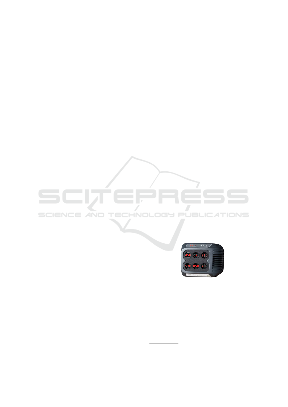
The multi-spectral imagery is provided by the six-

band multi-spectral camera Airphen developed by

HiPhen. Airphen is a scientiﬁc multi-spectral cam-

era developed by agronomists for agricultural appli-

cations. It can be embedded in different types of plat-

forms such as UAV, phenotyping robots, etc.

Airphen is highly conﬁgurable (bands, ﬁelds

of view), lightweight and compact. The camera

was conﬁgured using interferential ﬁlter centered at

450/570/675/710/730/850 nm with FWHM

of 10

nm, the position of each band is referenced on ﬁg-

ure 1. The focal lens is 8 mm for all wavelength. The

raw resolution for each spectral band is 1280 × 960

px with 12 bit of precision. Finally the camera also

provides an internal GPS antenna that can be used to

get the distance from the ground.

Figure 1: Disposition of each band on the Airphen multi-

sensors camera.

2.1.2 Datasets

Two datasets were taken at different heights with im-

ages of a chessboard (use for calibration) and of an

agronomic scene. We used a metallic gantry for po-

sitioning the camera at different heights. The size of

the gantry is 3 × 5 × 4 m. Due to the size of the chess-

board (57 × 57 cm with 14 × 14 square of 4 cm), the

Full Width at Half Maximum

VISAPP 2020 - 15th International Conference on Computer Vision Theory and Applications

104

limited focus of the camera and the gantry height, we

have bounded the acquisition heights from 1.6 to 5 m

with 20 cm steps, which represents 18 acquisitions.

The ﬁrst dataset is for the calibration. A chess-

board is taken at different heights The second one is

for the alignment veriﬁcation under real conditions.

One shot of an agronomic scene is taken at different

heights with a maximum bias set at 10 cm.

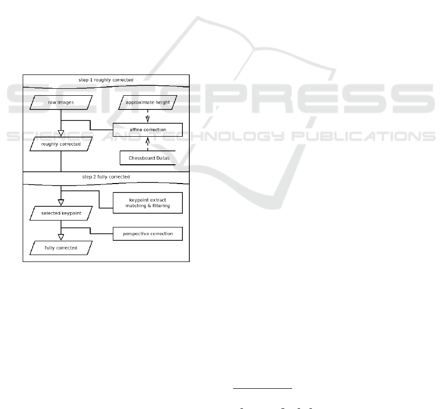
2.2 Methods

Alignment is reﬁned in two stages, with (i) afﬁne reg-

istration approximately estimated and (ii) perspective

registration for the reﬁnement and precision. As ex-

ample the ﬁgure 2 shows each correction step, where

the ﬁrst line is for the (i) afﬁne correction (section

2.2.1), the second is for (ii) perspective correction.

More precisely the second step is per-channel pre-

processed where feature detectors are used to de-

tect key-points (section 2.2.2). Each channel key-

points are associated to compute the perspective cor-

rection through homography, to the chosen spectral

band (section 2.2.2). These steps are explained on

speciﬁc subsections.

Figure 2: Each step of the alignment procedure, with (step

1) roughly corrected from afﬁne correction and (step 2) en-

hancement via key-points and perspective.

2.2.1 Afﬁne Correction

We make the assumption that closer we take the snap-

shot, the bigger the distance between each spectral

band is. On the other hand, at a distance superior

or equals to 5 m, the initial afﬁne correction become

stable. A calibration is used to build a linear model

based on that assumption, which will allow the afﬁne

correction to work at any height. The main purpose of

this step is to reduce the offset between each spectral

band, which allows the similarity between key-points

to be spatially delimited within a few pixels, making

feature matching more effective.

Calibration: Based on that previous assumption a

calibration is run over the chessboard dataset. We de-

tect the chessboard using the opencv calibration tool-

box (Bouguet, 2001) on each spectral image (nor-

malized by I = (I − min(I))/ max(I) where I is the

spectral image) at different heights (from 1.6 m to 5

m). We use the function ﬁndChessboardCorners how

attempts to determine whether the input image is a

view of the chessboard pattern and locate the inter-

nal chessboard corners. The detected coordinates are

roughly approximated. To determine their positions

accurately we use the function cornerSubPix as ex-

plained in the documentation

Linear Model: Using all the points detected for

each spectral band, we calculate the centroid grid

(each point average). The afﬁne transform from each

spectral band to this centroid grid is estimated. The-

oretically, the rotation and the scale (A,B,C,D) do

not depend on the distance to the ground, but the

translation (X,Y ) does. Thus a Levenberg-Marquardt

curve ﬁtting algorithm with linear least squares re-

gression (Mor

e, 1978) can be used to ﬁt an equation

for each spectral band against X and Y independently

to the centroid grid. We adjust the following curve

t = αh

+ βh

+ θh + γ where h is the height, t is the

resulted translation and factors α,β,θ,γ are the model

parameters.

Correction: Based on the model estimated on the

chessboard dataset, we transpose them to the agro-

nomic dataset. To make the afﬁne matrix correction,

we used the rotation and scale factors at the most ac-

curate height (1.6 m where the spatial resolution of

the chessboard is higher), because it does not theoret-

ically depend on the height. For the translation part,

the curve model is applied for each spectral band at

the given height provided by the user. Each spec-

tral band is warped using the corresponding afﬁne

transformation. Finally, all spectral bands are cropped

to the minimal bounding box (minimal and maximal

translation of each afﬁne matrix). This ﬁrst correction

is an approximation. It provides some spatial proper-

ties that we will use on the second stage.

https://docs.opencv.org/2.4/modules/calib3d/doc/came

ra calibration and 3d reconstruction.html

Two-step Multi-spectral Registration Via Key-point Detector and Gradient Similarity: Application to Agronomic Scenes for Proxy-sensing

105

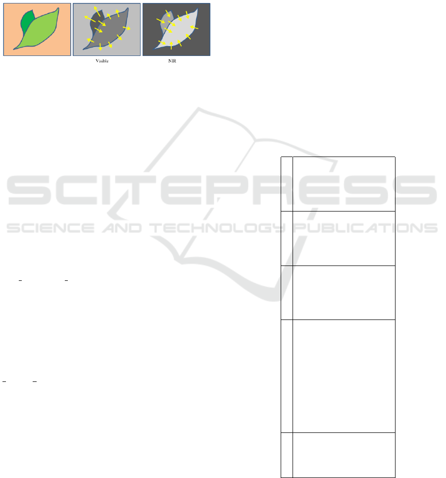
2.2.2 Perspective Correction

Each spectral band has different properties and values

by nature but we can extract the corresponding simi-

larity by transforming each spectral band into its ab-

solute derivative, to ﬁnd similarities in gradient break

among them. As we can see in ﬁgure 3 gradients

can have opposite direction depending on the spectral

bands, making the absolute derivative an important

step for matching between different spectral band.

Figure 3: Gradient orientation in spectral band (Rabatel and

Labbe, 2016). Orientation of the gradient is not the same

depending to the spectral band.

The afﬁne correction attempts to help the fea-

ture matching by adding properties of epipolar lines

(close). Thus, the matching of extracted features can

be spatially bounded, (i) we know that the maximum

translation is limited to a distance of a few pixels (less

than 10px thanks to afﬁne correction), and (ii) the an-

gle between the initial and the matched one is limited

to [−1,1] degree.

Computing the Gradient: To compute the gra-

dient of the image with a minimal impact of the

light distribution (shadow, reﬂectance, specular, ...),

each spectral band is normalized using Gaussian blur

(Sage and Unser, 2003), the kernel size is deﬁned by

next odd(image width

0.4

) (19 in our case) and the ﬁ-

nal normalized images are deﬁned by I/(G + 1) ∗ 255

where I is the spectral band and G is the Gaussian blur

of those spectral bands. This ﬁrst step minimizes the

impact of the noise on the gradient and smooth the

signal in case of high reﬂectance. Using this normal-

ized image, the gradient I

grad

(x,y) is computed with

the sum of absolute Sharr ﬁlter (Seitz, 2010) for hori-

zontal S

and vertical S

derivative, noted I

grad

(x,y) =

| +

|. Finally, all gradients I

grad

(x,y) are nor-

malized using CLAHE (Zuiderveld, 1994) to locally

improve their intensity and increase the number of

key-points detected.

Key-points Extractor: A key-point is a point of in-

terest. It deﬁnes what is important and distinctive in

an image. Different types of key-point extractors are

available and the following are tested :

(ORB) Oriented FAST and Rotated BRIEF

(Rublee et al., 2011), (AKAZE) Fast explicit diffu-

sion for accelerated features in nonlinear scale spaces

(Alcantarilla and Solutions, 2011), (KAZE) A novel

multi-scale 2D feature detection and description algo-

rithm in nonlinear scale spaces (Ordonez et al., 2018),

(BRISK) Binary robust invariant scalable key-points

(Leutenegger et al., 2011), (AGAST) Adaptive and

generic corner detection based on the accelerated seg-

ment test (Mair et al., 2010), (MSER) maximally sta-

ble extremal regions (Donoser and Bischof, 2006),

(SURF) Speed-Up Robust Features (Bay et al., 2006),

(FAST) FAST Algorithm for Corner Detection (Tra-

jkovi

c and Hedley, 1998) and (GFTT) Good Features

To Track (Shi et al., 1994).

These algorithms are largely described across

multiple studies (Dantas Dias Junior et al., 2019;

Tareen and Saleem, 2018; Zhang et al., 2016; Ali

et al., 2016), they are all available and easily usable

in OpenCV. Thus we have studied them by varying

the most inﬂuential parameters for each of them with

three modalities, the table 1 in appendix shows all

modalities.

Table 1: list of algorithms with 3 modalities of their param-

eters.

ABRV parameters modality 1 modality 2 modality 3

ORB nfeatures 5000 10000 15000

GFTT maxCorners 5000 10000 15000

AGAST threshold 71 92 163

FAST threshold 71 92 163

AKAZE nOctaves, nOctaveLayers (1, 1) (2, 1) (2, 2)

KAZE nOctaves, nOctaveLayers (4, 2) (4, 4) (2, 4)

BRISK nOctaves, patternScale (0, 0.1) (1, 0.1) (2, 0.1)

SURF nOctaves, nOctaveLayers (1, 1) (2, 1) (2, 2)

MSER None None None None

VISAPP 2020 - 15th International Conference on Computer Vision Theory and Applications

106

Key-point Detection: We use one of the key-point

extractors mentioned above between each spectral

band gradients (all extractors are evaluated). For each

detected key-point, we extract a descriptor using ORB

features. We match all detected key-points to a ref-

erence spectral band (all bands are evaluated). All

matches are ﬁltered by distance, position and angle,

to eliminate a majority of false positives along the

epipolar line. Finally we use the function ﬁndHomog-

raphy between the key-points detected/ﬁltered with

RANSAC (Fischler and Bolles, 1981), to determine

the best subset of matches to calculate the perspective

correction.

Correction: The perspective correction between

each spectral band to the reference is estimated and

applied. Finally, all spectral bands are cropped to the

minimum bounding box, which is obtained by apply-

ing a perspective transformation to each corner of the

image.

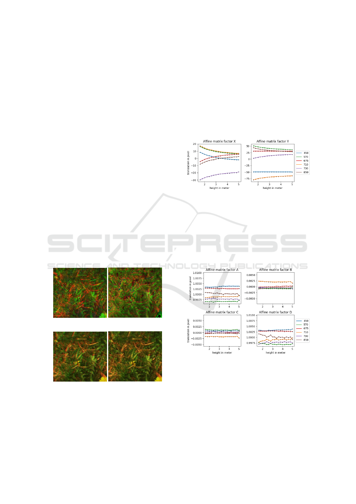
3 RESULTS AND DISCUSSION

Firstly the results will focus on afﬁne corrections and

then on the effects of the perspective correction. Fig-

ure 4 shows a closeup inside at 1.6 m (4a) raw images

acquisition, (4c & 4d) registred image of each correc-

tion steps and (4b) the manufacturer results.

(a) raw image (b) manufacturer’s

Figure 4: Example of each correction and the manufacturers

results.

3.1 Afﬁne Correction

The afﬁne correction model is based on the calibration

dataset (where the chessboard are acquired). The 6

coefﬁcients (A,B,C,D, X,Y ) of the afﬁne matrix were

studied according to the height of the camera in or-

der to see their stability. It appears that the translation

part (X,Y ), depends on the distance to the ﬁeld (ap-

pendix ﬁgure 5) according to the initial assumption.

On this part the linear model is used to estimate the

afﬁne correction from an approximated height.

Figure 5: Afﬁne matrix value by height.

Rotation and scale do not depend on the ground

distance (ﬁgure 6) according to the theory. These fac-

tors (A,B,C, D) are quite stable and close to identity,

as expected (accuracy depends on the spatial resolu-

tion of the board). As result, single calibration can be

used for this part of the matrix, and the most accurate

are used (i.e where the chessboard has the best spatial

resolution).

Figure 6: Afﬁne matrix value by height.

After the afﬁne correction, the remaining residual

distances have been extracted, it is computed using

the detected, ﬁltered and matched key-point to the ref-

erence spectral band, ﬁgure 9 (up) shows an example

using 570 nm as reference before the perspective cor-

rection. The remaining distance between each spec-

tral band to the reference varies according to the dis-

tance between the real height and the nearest selected

(through linear model). Remember that a bias of +/-

Two-step Multi-spectral Registration Via Key-point Detector and Gradient Similarity: Application to Agronomic Scenes for Proxy-sensing

107

10cm was initially set to show the error in the worst

case, so the difference of errors between each of them

are due to the difference of sensors position in the

array to the reference and the provided approximate

height.

3.2 Perspective Correction

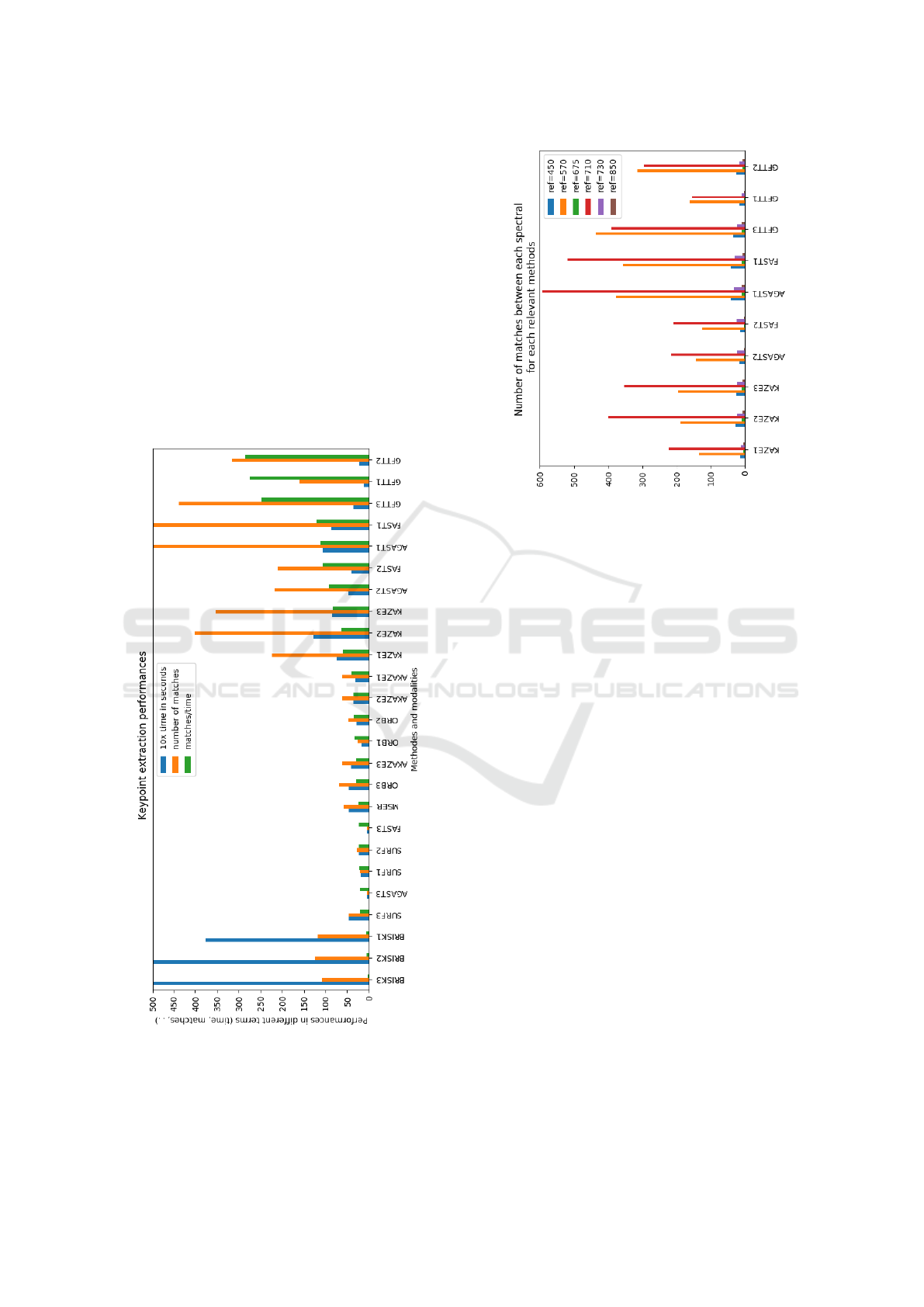
The ﬁgures 7 shows the numbers of key-points after

ﬁltering and homographic association (minimum of

all matches) as well as the computation time and per-

formance ratio (matches/time) for each method. The

performance ratio is used to compare methods be-

tween them, bigger he is, greater is the method (bal-

anced between time and accuracy), making lower of

them unsuitable.

Figure 7: Features extractor performances after ﬁltering and

homography association.

All these methods offer interesting results, the

choice of method depends on application needs be-

Figure 8: Key-point extractor performances.

tween computation time and accuracy, three methods

stand out in all of there modality:

• GFTT shows the best overall performance in both

computation time and number of matches

• FAST and AGAST1 are quite suitable too, with

acceptable computation time and greater matches

performances.

The other ones did not show improvement in term

of time or matches (especially compared to GFTT),

some of them show a small number of matches which

can be too small to ensure the precision. Increasing

the number of key-points matched allows a slightly

higher accuracy (Dantas Dias Junior et al., 2019). For

example, switching from SURF (30 results) to FAST

(130 results) reduces the ﬁnal residual distances from

≈ 1.2 to ≈ 0.9 px but increases the calculation time

from ≈ 5 to ≈ 8 seconds.

All methods show that the best spectral band is

710 nm (in red), with an exception for SURF and

GFTT which is 570 nm. The ﬁgure 8 shows the

minimum number of matches between each reference

spectrum and all the others, for each relevant meth-

ods and modalities (KAZE, AGAST, FAST GFTT).

Choosing the right spectral reference is important, as

we can see, no correspondence is found in some cases

between 675-850 nm, but correspondences are found

between 675-710 nm and 710-850 nm, making the

710 nm more appropriate, the same behavior can be

observed for the other bands and 570 nm as the more

appropriate one. This is visible on the ﬁgure for all

methods, 570 nm and 710 nm have the best minimum

number of matches where all the other are quite small.

VISAPP 2020 - 15th International Conference on Computer Vision Theory and Applications

108

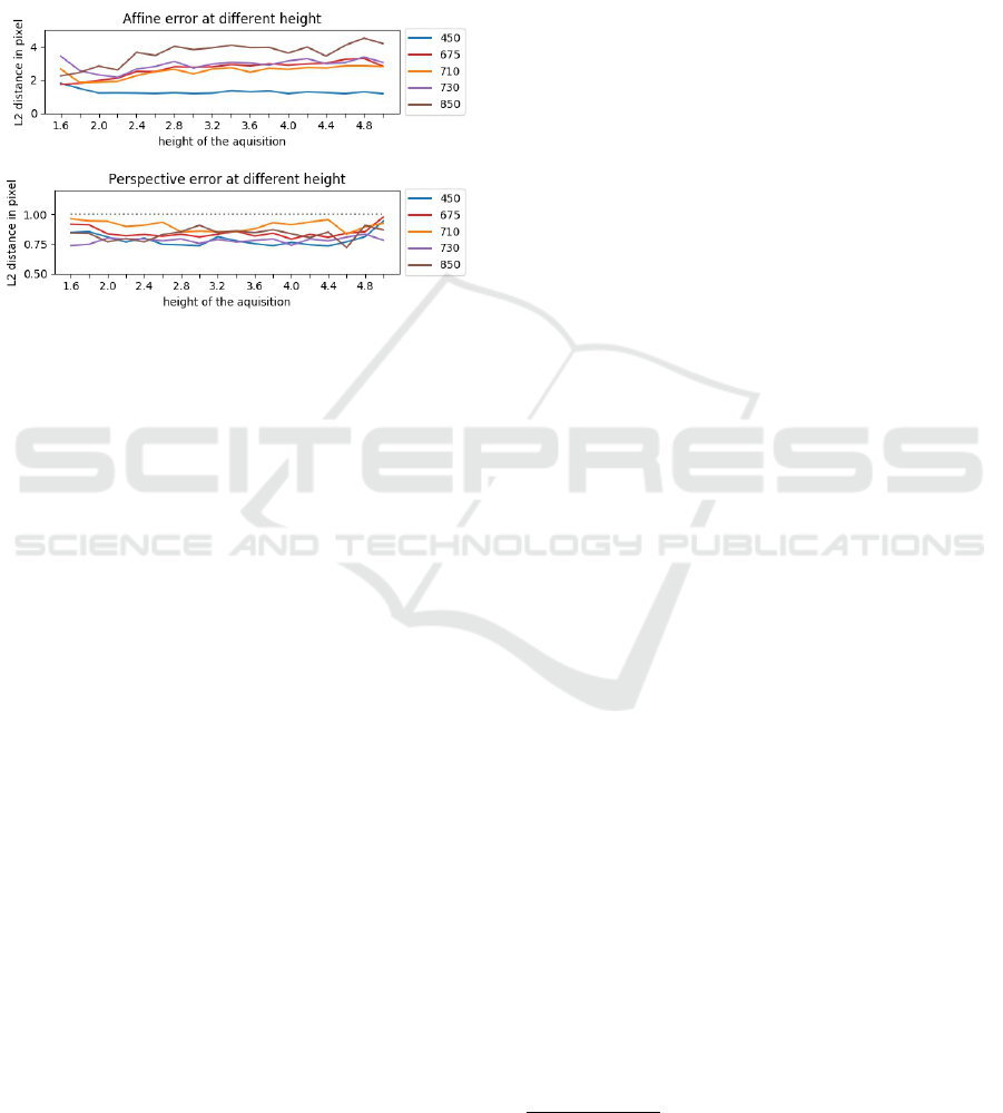
Residues of the perspective correction show that

we have correctly registered each spectral band, the

ﬁgure 9 (down) shows the residual distance at differ-

ent ground distances. In comparison the afﬁne correc-

tion error are between [1.0 −4.8] px where the combi-

nation of afﬁne and perspective correction the resid-

ual error are between [0.7 − 1.0] px. On average the

perspective correction enhance the residual error by

(3.5 − 0.9)/3.5 ≈ 74%.

Figure 9: (up) The mean distance of detected key-point be-

fore perspective correction with 570 nm as spectral refer-

ence (down) Perspective re-projection error with GFTT us-

ing the ﬁrst modality and 570 nm as reference.

3.3 General Discussion

Even if the relief of the scene is not taken into ac-

count due to the used deformation model, in our case,

with ﬂat ground, no difference arise. However, more

complex deformation models (Lombaert et al., 2012;

Bookstein, 1989) could be used to improve the re-

maining error. But could also, in some case, create

large angular deformations caused by the proximity

of key-points, of course, it’s possible to ﬁlter these

key-points, which would also reduce the overall accu-

racy.

Further research can be performed on each pa-

rameter of the feature extractors, for those who need

speciﬁc performance (time/precision), we invite any-

one to download the dataset and test various combina-

tions. Otherwise feature matching can be optimized,

at this stage, we use brute-force matching with post

ﬁltering, but a different implementation that fulﬁll our

spatial properties should greatly enhance the number

of matches by reducing false positives.

4 CONCLUSION

In this work, the application of different techniques

for multi-spectral image registration was explored us-

ing the Airphen camera. We have tested nine type

of key-points extractor (ORB, GFTT, AGAST, FAST,

AKAZE, KAZE, BRISK, SURF, MSER) at different

heights and the number of control points obtained. As

seen in the method, the most suitable method is the

GFTT (regardless of modalities 1, 2 or 3) with a sig-

niﬁcant number of matches 150 − 450 and a reason-

able calculation time 1.17 s to 3.55 s depending on the

modality.

Furthermore, the best spectral reference was de-

ﬁned for each method, for example 570 nm for GFTT.

We have observed a residual error of less than 1 px,

supposedly caused by the difference of sensors nature

(spectral range, lens).

ACKNOWLEDGMENTS

The authors acknowledge support from European

Union through the project H2020 IWMPRAISE

(Integrated Weed Management: PRActical Im-

plementation and Solutions for Europe) and from

ANR Challenge ROSE through the project ROSEAU

(RObotics SEnsorimotor loops to weed AU-

tonomously).

We would like to thanks Combaluzier Quentin,

Michon Nicolas, Savi Romain and Masson Jean-

Benoit for the realization of the metallic gantry that

help us positioning the camera at different heights.

REFERENCES

Alcantarilla, P. F. and Solutions, T. (2011). Fast ex-

plicit diffusion for accelerated features in nonlinear

scale spaces. IEEE Trans. Patt. Anal. Mach. Intell,

34(7):1281–1298.

Ali, F., Khan, S. U., Mahmudi, M. Z., and Ullah, R. (2016).

A comparison of fast, surf, eigen, harris, and mser fea-

tures. International Journal of Computer Engineering

and Information Technology, 8(6):100.

Bay, H., Tuytelaars, T., and Van Gool, L. (2006). Surf:

Speeded up robust features. In European conference

on computer vision, pages 404–417. Springer.

Bookstein, F. L. (1989). Principal warps: thin-plate splines

and the decomposition of deformations. IEEE Trans-

actions on Pattern Analysis and Machine Intelligence,

11(6):567–585.

Bouguet, J.-Y. (2001). Camera calibration toolbox for mat-

lab.

Chen, S., Shen, H., Li, C., and Xin, J. H. (2018). Normal-

ized total gradient: A new measure for multispectral

image registration. IEEE Transactions on Image Pro-

cessing, 27(3):1297–1310.

https://iwmpraise.eu/

http://challenge-rose.fr/en/projet/roseau-2/

Two-step Multi-spectral Registration Via Key-point Detector and Gradient Similarity: Application to Agronomic Scenes for Proxy-sensing

109

Dantas Dias Junior, J., Backes, A., and Escarpinati,

M. (2019). Detection of control points for uav-

multispectral sensed data registration through the

combining of feature descriptors. pages 444–451.

Donoser, M. and Bischof, H. (2006). Efﬁcient maximally

stable extremal region (mser) tracking. In 2006 IEEE

Computer Society Conference on Computer Vision

and Pattern Recognition (CVPR’06), volume 1, pages

553–560. Ieee.

Douarre, C., Crispim-Junior, C. F., Gelibert, A., Tougne,

L., and Rousseau, D. (2019). A strategy for mul-

timodal canopy images registration. In 7th Interna-

tional Workshop on Image Analysis Methods in the

Plant Sciences, Lyon, France.

Fischler, M. A. and Bolles, R. C. (1981). Random sample

consensus: A paradigm for model ﬁtting with appli-

cations to image analysis and automated cartography.

Commun. ACM, 24(6):381–395.

Jin, X.-l., Diao, W.-y., Xiao, C.-h., Wang, F.-y., Chen,

B., Wang, K.-r., and Li, S.-k. (2013). Estimation of

wheat agronomic parameters using new spectral in-

dices. PLOS ONE, 8(8):1–9.

Kamoun, E. (2019). Image registration: From sift to deep

learning.

Lechenet, M., Bretagnolle, V., Bockstaller, C., Boissinot,

F., Petit, M.-S., Petit, S., and Munier-Jolain, N. M.

(2014). Reconciling pesticide reduction with eco-

nomic and environmental sustainability in arable

farming. PLOS ONE, 9(6):1–10.

Leutenegger, S., Chli, M., and Siegwart, R. (2011). Brisk:

Binary robust invariant scalable keypoints. In 2011

IEEE international conference on computer vision

(ICCV), pages 2548–2555. Ieee.

Lombaert, H., Grady, L., Pennec, X., Ayache, N., and

Cheriet, F. (2012). Spectral demons – image registra-

tion via global spectral correspondence. In Fitzgib-

bon, A., Lazebnik, S., Perona, P., Sato, Y., and

Schmid, C., editors, Computer Vision – ECCV 2012,

pages 30–44, Berlin, Heidelberg. Springer Berlin Hei-

delberg.

Mair, E., Hager, G. D., Burschka, D., Suppa, M., and

Hirzinger, G. (2010). Adaptive and generic corner de-

tection based on the accelerated segment test. In Euro-

pean conference on Computer vision, pages 183–196.

Springer.

Mor

e, J. J. (1978). The levenberg-marquardt algorithm:

Implementation and theory. In Watson, G., editor,

Numerical Analysis, volume 630 of Lecture Notes in

Mathematics, pages 105–116. Springer Berlin Heidel-

berg.

Ordonez, A., Arguello, F., and Heras, D. B. (2018). Align-

ment of hyperspectral images using kaze features. Re-

mote Sensing, 10(5).

Rabatel, G. and Labbe, S. (2016). Registration of visi-

ble and near infrared unmanned aerialvehicle images

based on Fourier-Mellin transform. Precision Agri-

culture, 17(5):564–587.

Rublee, E., Rabaud, V., Konolige, K., and Bradski, G.

(2011). Orb: An efﬁcient alternative to sift or surf. In

Proceedings of the 2011 International Conference on

Computer Vision, ICCV ’11, pages 2564–2571, Wash-

ington, DC, USA. IEEE Computer Society.

Sage, D. and Unser, M. (2003). Teaching image-processing

programming in java. IEEE Signal Processing Maga-

zine, 20(6):43–52. Using “Student-Friendly” ImageJ

as a Pedagogical Tool.

Sankaran, S., Khot, L. R., Espinoza, C. Z., Jarolmasjed,

S., Sathuvalli, V. R., Vandemark, G. J., Miklas, P. N.,

Carter, A. H., Pumphrey, M. O., Knowles, N. R., and

Pavek, M. J. (2015). Low-altitude, high-resolution

aerial imaging systems for row and ﬁeld crop pheno-

typing: A review. European Journal of Agronomy,

70:112 – 123.

Seitz, H. (2010). Contributions to the minimum linear ar-

rangement problem.

Shi, J. et al. (1994). Good features to track. In 1994 Pro-

ceedings of IEEE conference on computer vision and

pattern recognition, pages 593–600. IEEE.

Tareen, S. A. K. and Saleem, Z. (2018). A comparative

analysis of sift, surf, kaze, akaze, orb, and brisk. 2018

International Conference on Computing, Mathemat-

ics and Engineering Technologies (iCoMET), pages

1–10.

Trajkovi

c, M. and Hedley, M. (1998). Fast corner detection.

Image and vision computing, 16(2):75–87.

Vakalopoulou, M. and Karantzalos, K. (2014). Automatic

descriptor-based co-registration of frame hyperspec-

tral data. Remote Sensing, 6.

Vioix, J.-B. (2004). Conception et r

ealisation d’un dispositif

d’imagerie multispectrale embarqu

e : du capteur aux

traitements pour la d

etection d’adventices.

Zhang, H., Wohlfeil, J., and Grießbach, D. (2016). Exten-

sion and evaluation of the agast feature detector.

Zitov

a, B. and Flusser, J. (2003). Image registration meth-

ods: A survey. Image and Vision Computing, 21:977–

1000.

Zuiderveld, K. (1994). Contrast limited adaptive histogram

equalization. In Graphics gems IV, pages 474–485.

Academic Press Professional, Inc.

VISAPP 2020 - 15th International Conference on Computer Vision Theory and Applications

110