
Visualizing Learning Space in Neural Network Hidden Layers
Gabriel D. Cantareira
1
, Fernando V. Paulovich
2
and Elham Etemad
2
1
Universidade de S
˜
ao Paulo, Brazil
2
Dalhousie University, Canada
Keywords:
Machine Learning, Neural Network Visualization, Deep Neural Networks.
Abstract:
Analyzing and understanding how abstract representations of data are formed inside deep neural networks is a
complex task. Among the different methods that have been developed to tackle this problem, multidimensional
projection techniques have attained positive results in displaying the relationships between data instances,
network layers or class features. However, these techniques are often static and lack a way to properly keep a
stable space between observations and properly convey flow in such space. In this paper, we employ different
dimensionality reduction techniques to create a visual space where the flow of information inside hidden layers
can come to light. We discuss the application of each used tool and provide experiments that show how they
can be combined to highlight new information about neural network optimization processes.
1 INTRODUCTION
Given their ability to abstract high-level patterns and
model data beyond most heuristics (LeCun et al.,
2015), deep neural networks (DNNs) are currently
among the state-of-the-art techniques for the analysis
of large-scale, complex datasets. Despite the preva-
lence of DNNs in different domains, such as natu-
ral language processing, face and speech recognition,
and generation of artificial data, its success heavily
depends on the right choice of hyperparameters and
architecture.
In recent years, visualization strategies have be-
come increasingly popular in the research commu-
nity to help analysts interpret the results and support
the improvement of DNNs. One of the most popular
visualization strategies, multidimensional projection
techniques (Nonato and Aupetit, 2018) have report-
edly attained relative success in helping users to ex-
plore and explain what happens inside DNNs (Rauber
et al., 2017; Mahendran and Vedaldi, 2015; Srivastava
et al., 2014). These techniques aim to generate lower-
dimensional visual representations of the data capable
of preserving data structure, such as relationships be-
tween data instances or the presence of clusters. How-
ever, the currently available techniques are somewhat
limited when exploring sequential processes inside
the network, such as the state of hidden layers during
training or the shaping of high-level representations
as data flows through different layers of a network.
In this paper, we present a novel approach to visu-
alize the hidden structure of DNNs that aids in under-
standing the generated abstract high-level represen-
tations and how they are formed during the training
process. In our approach, we employ different tech-
niques to project data extracted from various states
of a neural network and estimate a common space
that can show how these projections relate to one an-
other by computing a vector field from the projected
data. Based on these methods, we show possibili-
ties in identifying flow and tracking down meaningful
changes in the neural network as abstract representa-
tions of data are formed.
Our main contributions are:
• A projection-based visual representation better
suited to represent sequential aspects of DNNs,
eliminating movement clutter while keeping dis-
tances meaningful;
• A visual transition space between two or more
sequential projections that is not restricted by a
varying number of dimensions of the input data.
2 RELATED WORK
Artificial neural networks (ANNs) are structures com-
posed of groups of simple and complex cells. Sim-
ple cells are responsible for extracting basic features,
while complex ones combine local features producing
110
Cantareira, G., Paulovich, F. and Etemad, E.
Visualizing Learning Space in Neural Network Hidden Layers.
DOI: 10.5220/0009168901100121
In Proceedings of the 15th International Joint Conference on Computer Vision, Imaging and Computer Graphics Theory and Applications (VISIGRAPP 2020) - Volume 3: IVAPP, pages
110-121
ISBN: 978-989-758-402-2; ISSN: 2184-4321
Copyright
c
2022 by SCITEPRESS – Science and Technology Publications, Lda. All rights reserved

abstract representations (Scherer et al., 2010). This
structure hierarchically manipulates data through lay-
ers (complex cells), each one using a set of process-
ing units or neurons (simple cells) to extract local
features. In classification tasks, each neuron divides
input data space using a linear function (i.e., hyper-
plane), which is positioned to obtain the best sepa-
ration as possible between labels of different classes.
Thus, the connections among processing units are re-
sponsible for combining the half-spaces built up by
those linear functions to produce nonlinear separabil-
ity of data spaces (LeCun et al., 2015). Deep neural
networks (DNNs) are artificial neural network mod-
els that contain a large number of layers between in-
put and output, generating more complex representa-
tions. Such networks are called convolutional neural
networks (CNNs) when convolutional filters are em-
ployed.
In the past few years, the use of visualization tools
and techniques to support the understanding of neu-
ral network models has become more prolific, with
many different approaches focusing on exploring and
explaining different aspects of DNN training, topol-
ogy, and parametrization (Hohman et al., 2018). As
deep models grow more complex and sophisticated,
understanding what happens to data inside these sys-
tems is quickly becoming key to improving their effi-
ciency and designing new solutions.
When exploring layers of a DNN, a common
source of data is the hidden layer activations: the out-
put value of each neuron of a given layer when sub-
jected to a data instance (input). Many DNN visual-
ization approaches are focused on understanding the
high-level abstract representations that are formed in
hidden layers. This is often attained by transferring
the activations of hidden layer neurons back to the
feature space, as defined by the Deconvnet (Zeiler and
Fergus, 2014) and exemplified by applications such as
the Deep Dream (Szegedy et al., 2015). Commonly
associated with CNNs, techniques based on this ap-
proach often try to explain and represent which fea-
ture values in a data object generate activations in
certain parts of hidden layers. The Deconvnet is capa-
ble of reconstructing input data (images) at each CNN
layer to show the features extracted by filters, support-
ing the detection of incidental problems based on user
inspections.
Other techniques focus on identifying content that
activates filters and hidden layers. Simonyan et
al. (Simonyan et al., 2013) developed two visualiza-
tion tools based on Deconvnet to support image seg-
mentation, allowing feature inspection and summa-
rization of produced features. Zintgraf et al. (Zintgraf
et al., 2017) introduced a feature-based visualization
tool to assist in determining the impact of filter size
on classification tasks and identifying how the deci-
sion process is conducted. Erhan et al. (Erhan et al.,
2009) proposed a strategy to identify features detected
by filters after their activation functions, allowing the
visual inspection of the impact of network initializa-
tion as well as if features are humanly understandable.
Similarly, Mahendran et al. (Mahendran and Vedaldi,
2016) presented a triple visualization analysis method
to inspect images. Babiker et al. (Babiker and Goebel,
2017) also proposed a visual tool to support the iden-
tification of unnecessary features filtered in the layers.
Liu et al. (Liu et al., 2017) present a system capable
of showing a CNN as an acyclic graph with images
describing each filter.
Other methods aim to explore the effects of differ-
ent parameter configurations in training, such as reg-
ularization terms or optimization constraints (Srivas-
tava et al., 2014). These can also be connected to dif-
ferent results in layer activations or classification out-
comes. Some techniques are designed to help evalu-
ate the effectiveness of specific network architectures,
estimating what kind of abstraction can be learned
in each section, such as the approach described by
Yosinki et al. (Yosinski et al., 2015).
The research previously described is focused on
identifying and explaining what representations are
generated. However, it is also important to under-
stand how those representations are formed, regard-
ing both the training process and the flow of infor-
mation inside a network. Comprehending these as-
pects can lead to improvements in network archi-
tecture and the training process itself. The Deep-
Eyes framework, developed by Pezzotti et al.(Pezzotti
et al., 2018), provides an overview of DNNs, being
capable of identifying when a network architecture
requires more or fewer filters or layers, employing
scatterplots and heatmaps to show filter activations
and allowing the visual analysis of the feature space.
Kahng et al. (Kahng et al., 2018) introduce a method
to explore the features produced by CNNs project-
ing activation distances and presenting a neuron ac-
tivation heatmap for specific data instances. These
techniques are, however, not designed for projecting
multiple transition states and their projection methods
require complex parametrization to show the desired
information.
Multidimensional projections (or dimensionality
reduction techniques) (Nonato and Aupetit, 2018) are
popular tools to aid the study of how abstract rep-
resentations are generated inside ANNs. Specific
projection techniques, such as the UMAP (McInnes
et al., 2018), were developed particularly with ma-
chine learning applications in mind. While dimen-
Visualizing Learning Space in Neural Network Hidden Layers
111

sionality reduction techniques are generally used in
ANN studies to illustrate model efficacy (Donahue
et al., 2014; Srivastava et al., 2014; Hamel and Eck,
2010; Mohamed et al., 2012; Mahendran and Vedaldi,
2015), Rauber et Al (Rauber et al., 2017) showed their
potential on providing valuable visual information on
DNNs to improve models and observe the evolution
of learned representations. Projections were used to
reveal hidden layer activations for test data before and
after training, highlighting the effects of training, the
formation of clusters, confusion zones, as well as the
neurons themselves, using individual activations as
attributes. Despite offering insights on how the net-
work behaves before and after training, the visual rep-
resentation presented by the authors for the evolution
of representations inside the network or the effects
of training between epochs displays a great deal of
clutter; when analyzing a large number of transition
states, information such as the relationships between
classes or variations that occur only during intermedi-
ate states may become difficult to infer. Additionally,
the method used to ensure that all projections share
a similar 2D space is prone to problems in alignment
and performance. In this paper, we propose a visual-
ization scheme that employs a flow-based approach to
offer a representation better suited to show transition
stated and evolving data in DNNs. We also briefly
address certain pitfalls encountered when visualizing
neuron activation data using standard projection tech-
niques, such as the t-SNE (Van Der Maaten and Hin-
ton, 2008), and discuss why these pitfalls are relevant
to our application.
3 VISUALIZING LEARNING
SPACE
Our visual representation is based on gathering layer
activation data from a sequence of ANN outputs, then
projecting them onto a 2D space while sharing infor-
mation to ensure semantically similar data remain in
similar positions between projections. The movement
of the same data instance between projections gener-
ate trajectories, which are then condensed into vector
fields that reflect how data flows throughout the differ-
ent outputs. These outputs consist of layer activations,
either from a specific layer during different epochs of
training (to visualize how training changes data rep-
resentations), or from different layers from the same
instance of a network (to visualize how data represen-
tations evolve as layers propagate information.
To build this representation, we first extract acti-
vation sets A(1), A(2), . . . , A(T ) representing the net-
work outputs from T sequential steps of the process
we want to explore. In this paper, we either a) save
the network model at different epochs of training,
choose a slicing layer, feed the same set of input data
to the saved models, and then save the outputs from
the layer, or b) pick a given network model, slice it at
different layers, feed the input data set, and save the
output from these layers as activation sets.
Once the activation data is extracted, it is pro-
jected onto a 2D space using a multidimensional pro-
jection technique, obtaining A
p
[1], A
p
[2], . . . , A
p
[T ].
Then, the positions of the same points in two sub-
sequent projections form movement vectors that de-
scribe how data instances in one output changed to
the next. This movement data is joined for all out-
put transitions, generating trajectories for each data
instance across the sequential steps we wanted to ex-
plore. Finally, all trajectories are used to compute a
vector field to explain and visualize how and what the
network has learned in the training process. The 2D
space shared by all projections is our visual learning
space, and the vector field describes how network out-
puts flow through it. Figure 1 summarizes this pro-
cess.
The following sections show in detail how data is
projected and how the vector field is generated in our
model.
3.1 Projecting Data
Although we can compare any set of projections to
produce vector fields, we need to eliminate changes
between projections that do not reflect variations
in the high-dimensional data as much as possible.
Therefore, the projection technique itself must share
information between all observations to ensure the
generation of a synchronized view. Although precise
and popular, non-linear projection techniques gener-
ally do not guarantee consistent visual spaces when
comparing two distinct projections since the axis (di-
mensions) of the original space are not projected into
straight lines on the visual spaces, and, therefore, can-
not be considered equivalent in the projections. Some
techniques offer a certain degree of control, such as
fixing control points (Joia et al., 2011) or selecting
the same initialization parameters (Van Der Maaten
and Hinton, 2008), but often this means a trade-off
between local and global distance preservation.
For two distinct projections to be compared, they
need to be aligned as best as possible, i.e., the pro-
jected distances must be as similar as possible to the
original data while keeping the projections as simi-
lar as possible with each other. Currently, there are
two techniques able to generate multiple aligned pro-
jections of the same data: the Dynamic t-SNE (Dt-
IVAPP 2020 - 11th International Conference on Information Visualization Theory and Applications
112
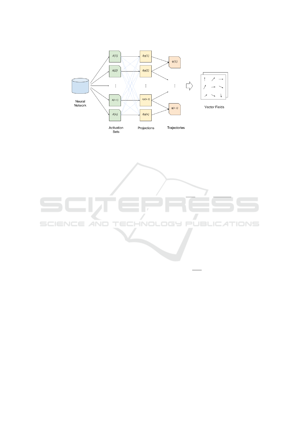
Figure 1: Overview of the learning space vector field generation. From the DNN model, we obtain sequential data, in the
form of hidden layer activations. From this highly multivariate data, we compute projections, sharing information between all
activation sets (dashed lines) to ensure that the obtained projections are synchronized. The differences between each pair of
projections in the sequence are then processed to obtain vector fields that represent the changes in data.
SNE) (Rauber et al., 2016) and the Visual Feature Fu-
sion (VFF) (Hilasaca and Paulovich, 2019).
The Dt-SNE is a variation of the t-SNE capable
of minimizing data variability in successive projec-
tions to a certain degree in order to observe changes
in multiple DNN states. This is achieved by adding a
term to the t-SNE’s cost function to approach points
representing the same instance in different projections
close to each other. Although attaining better results
if compared to the original t-SNE in terms of align-
ing subsequent projections, it inherits a major prob-
lem: the misleading effect of cluster distance and
shape in t-SNE projections resulted from the local
nature of the optimization and how hyperparameters
are set up (Wattenberg et al., 2016) – the observed
distance between clusters is unreliable and sensitive
to parametrization (perplexity parameter), conflicting
with our design goals.
Given that, we opt to use the VFF technique. VFF
is next described.
3.1.1 Aligning Projections
The VFF technique was originally developed to fuse
different feature representations of data with the aim
of building a new, user-driven representation. Here,
we use it to generate 2D projections that align differ-
ent feature representations of the same data.
This process consists of obtaining samples
F
1
, ..., F
T
from the activation sets A[1]...A[T ] with the
same indexes (i.e., the samples contain data related
to the same points) and then calculating representa-
tions R
1
, ..., R
T
∈ R
2
that preserves the relationships
in each set F
k
as best as possible while aligning the
projections. In this process, two restrictions are con-
sidered for optimization. The first is responsible for
ensuring that the projection matches the original data
and is given by
E
stress
(F
k
) =
1
|
F
k
|
2
|
F
k
|
∑
i
|
F
k
|
∑
j
δ( f
k
i
, f
k
j
)
δ
k
max
−
r
k
i
− r
k
j
!
2
(1)
where f
k
i
and f
k
j
are instances in F
k
, δ
f
k
i
, f
k
j
is the
distance between them on their original space, δ
k
max
is
the maximum pairwise distance between instances in
F
k
, and r
k
i
and r
k
j
are the representations of f
k
i
and f
k
j
on the m-dimensional space, respectively. The second
restriction is responsible for the alignment between
projections, given by
E
alignment
(F
k
) =
1
|
F
k
|
2
|
F
k
|
∑
i
|
F
k
|
∑
j
d(¯r
i
, ¯r
j
) −
¯r
i
− r
k
j
2
(2)
where d (¯r
i
, ¯r
j
) is the average distance between
two instances in all representations. Our experi-
ments were performed using Euclidian distances and
l
2
−norm, as we intend to visually examine distance
relations in the 2D space. This technique is, however,
designed to be able to merge features from different
distance metrics. Joining the two equations, the final
optimization problem is described by the equation
E(F
k
) = λ · E
stress
(F
k
) + (1 − λ) · E
alignment
(F
k
) (3)
where λ is a parameter used to control the importance
of each aspect of the optimization. This equation is
minimized using stochastic gradient descent.
Visualizing Learning Space in Neural Network Hidden Layers
113

3.2 Vector Field Generation
The vector fields contained in our visualization are
generated using an adapted version of the Vector Field
K-means technique, proposed by Ferreira et al. (Fer-
reira et al., 2013). This technique uses a distance mea-
sure d(X , a) between a discrete grid representation of
a vector field X and a trajectory a, composed by pairs
of time and spatial position (t, a(t)). Once this dis-
tance function is defined, it is minimized to find dis-
crete vector fields that provide the best approximation
to a group of trajectories and match each trajectory to
a field, similar to the k-means algorithm.
In this approach, a trajectory is represented by a
path written as α : [t
0
, t
1
] → R
n
and a vector field is de-
fined in a domain Ω ⊂ R
n
, i.e., a function X : Ω → R
n
.
So that, finding the vector field that best matches a set
of trajectories φ can be described as the optimization
problem
E = min
X
∑
α
i
∈φ
Z
t
i
1
t
i
0
X (α
i
(t)) −
α
0
(t)
2
dt (4)
where α
0
(t) is the velocity vector of the trajectory α
on instant t. Also included in this problem is a regu-
larization restriction
E = min
X
λ
L
k
∆X
k
2
+
(1 − λ
L
)
∑
α
i
∈φ
Z
t
i
1
t
i
0
(α
i
(t)) −
α
0
(t)
2
dt
(5)
where ∆ is the Laplace operator. This restriction en-
sures the smoothness of the resulting vector field, with
parameter λ
L
controlling the weight of each term in
the minimization equation and therefore determining
if the optimization should prioritize smoothness or
matching the vector field to the trajectories.
In the Vector Field k-Means technique, vector
fields are generated from trajectory groups, so that
trajectories can be reassigned to the most similar vec-
tor fields in the next half of the iteration. Since our
focus is to generate only one vector field that approx-
imates a set of trajectories, our simplified version of
this technique only fits the vector field to the trajec-
tory set, with no need for reassignment.
4 RESULTS
One typical application of DNNs is data classifica-
tion, which consists of inferring some model f : X →
Y to correctly label unknown data based on a set
of known labelled examples (x
i
, y
i
) ∈ X × Y (LeCun
et al., 2015). This learning process is known as su-
pervised learning, in which the model is iteratively
adapted according to training examples.
Although it is well established in the literature
that DNNs yield outstanding results in classification
tasks for different domains, training the network and
choosing appropriate parameters can still be a com-
plex, time-consuming process. In this section, we
visualize the projected learning space on MLPs and
CNNs performing classification tasks with the objec-
tive of gaining insights on the training process and on
how conclusions are drawn when performing classifi-
cation.
It is important to clarify that these visualization
methods are not restricted to a specific architecture or
application. These network configurations were cho-
sen due to their pervasiveness on literature, and be-
cause the classification problem offers an easy way to
keep track of instances by coloring the points repre-
senting them using the assigned classes.
4.1 Experimental Setup
In order to allow the comparison between our
approach and the results reported by Rauber et
al.(Rauber et al., 2017), we used the same network
configuration described in their experiments:
• An MLP with four fully-connected layers of
1, 000 rectified linear processing units (ReLU ac-
tivation) each, a 10 unit softmax output, and
dropout regularization of 0.2 − 0.5 on each hid-
den layer;
• A CNN consisting of two sequential convolu-
tional layers of 32 3 × 3 filters, a 2 × 2 max-
pooling layer (dropout 0.25), two convolutional
layers with 64 3 × 3 filters, another 2 × 2 max-
pooling layer (dropout 0.25), a fully-connected
layer with 4, 096 processing units (dropout 0.5),
a fully connected layer with 512 processing units,
and a softmax output with 10 units. All layers (ex-
cept the output) use ReLU activation.
Our experiments were conducted using the
CIFAR-10 and the MNIST datasets. Training opti-
mization was conducted using stochastic gradient de-
scent in both networks. In the MLPs, the employed
parameters were batch size equal to 16, learning
rate = 0.01, momentum coefficient = 0.9, and learn-
ing decay = 10
−9
. In the CNNs, the parameters were
batch size = 32, learning rate = 0.01, momentum coef-
ficient = 0.9, and learning decay = 10
−6
. We extracted
network snapshots after 0, 5, 10, and 100 training
epochs. The models for comparison between layers
IVAPP 2020 - 11th International Conference on Information Visualization Theory and Applications
114
are all based on networks after 100 training epochs.
Implementation is coded on CUDA-enabled Tensor-
Flow, using Keras
1
, NumPy
2
, and SciKit Learn
3
li-
braries. The vector field generation is based on the
code provided by Ferreira et al. (Ferreira et al., 2013),
and the visualization system was built using D3.js
4
.
For the projections, 2, 000 data instances were ran-
domly sampled from the test data of each dataset. We
used the same sample for all tests of the same dataset
to provide consistency. We produced hidden layer ac-
tivations by predicting the classes for the data sample
on all the snapshots of different training epochs and
capturing the results on the last hidden layer (1, 000
processing units on the MLP, 512 processing units on
the CNN). To compare different layers, we used the
trained network snapshots after 100 epochs and cap-
tured the results of each hidden layer on the MLP. On
the CNN, we captured results from 4 different layers:
the first max-pooling layer, the second max-pooling
layer, the first fully-connected layer, and the second
fully-connected layer. The filter information from the
convolutional layers was flattened and read as a vec-
tor. To project data, we used λ = 0.5.
Accuracy results for all training experiments can
be seen in Tables 1 and 2. There was a quick con-
vergence in the experiments done using the MNIST
dataset. The CIFAR10 experiments took longer and
got worse results, showing drops in accuracy due to
overfitting by epoch 100. It is important to mention
that in this paper, we do not seek the best accuracy
results in these tests - our goal is to explain why these
results happen. Therefore, while changes in accuracy
may seem small, we can explore these networks and
observe the fine tuning that is applied over the course
of 100 training epochs.
4.2 Evolution of Representations with
Training
Our first analysis was to observe hidden layer acti-
vations during training. We generated four visualiza-
tions, one for each dataset/network combination, each
composed by four projections, one for each training
epoch snapshot. Our goal was to compare the projec-
tions and identify useful information about the train-
ing process from the vector field model.
The results of the projections obtained for the
MNIST dataset can be seen in Figure 2. The MNIST
dataset is well-behaved compared to other image clas-
sification sets, and both networks achieved positive
1
keras.io
2
www.numpy.org
3
scikit-learn.org
4
www.d3js.org
Table 1: MNIST dataset accuracy using different network
architectures after e epochs.
network e = 5 e = 10 e = 100
MLP 0.9812 0.9823 0.9841
CNN 0.9933 0.9952 0.9954
rMLP 0.9806 0.9823 0.9849
Table 2: CIFAR10 dataset accuracy using different network
architectures after e epochs.
network e = 5 e = 10 e = 100
MLP 0.3260 0.3555 0.2803
CNN 0.6673 0.7538 0.7344
results (classification accuracy of 98% for the MLP
and 99% for the CNN). the projections show a high
level of separation right from the start: this is due to
the separability inherent to the data, even when mul-
tiplied by random weights. While the alignment pro-
cess also forces the first projection to be similar to the
later, better segmented ones, we also observed simi-
lar behavior even with very small λ values. The quick
optimization is reflected in the vector fields by a clear
outwards expansion as data instances are clustered in
their respective classes. It is possible to notice that
the expansion in the CNN is slightly more expressive
than the one observed in the MLP. This indicates a
quicker optimization process, as the CNN approaches
a high accuracy plateau slightly faster. The results of
this experiment are simple but demonstrate how our
approach can be used to show that both networks are
capable of solving the problem quite quickly, prob-
ably indicating that the employed architectures may
be excessive for the task. As further iterations group
the data in ever smaller sections of the visual space,
more caution should be advised to avoid overfitting.
As the number of instances and projection snapshots
increase in datasets, this visualization is able to pro-
vide information regarding convergence, transition
density, and temporal flow of data in a simpler and
cleaner way, compared to previous approaches.
Figure 3 shows the analysis of the CIFAR-10
dataset using both networks. The CIFAR-10 dataset is
much more complex and, therefore, more difficult to
classify when compared to the MNIST. The classifica-
tion results reflect this (accuracy of 35% for the MLP
and 75% for the CNN). The fact that the networks did
not yield particularly good results can lead to some
interesting observations. For instance, the clear out-
wards expansion observed in the vector fields on pre-
vious tests is absent in the MLP model and much less
pronounced in the CNN. Data still expands to a larger
area, but in a much more disorganized manner. Tra-
jectories of points heading in opposite directions may
Visualizing Learning Space in Neural Network Hidden Layers
115
Figure 2: Last hidden layer activation projections for the MNIST dataset on MLP (left) and CNN (right), with the obtained
vector fields on the lower part. The upper area shows the projections of activations from the last hidden layer after different
numbers of training epochs. The lower area shows the resulting vector fields of the transitions between the four projections.
As MNIST is a simpler, more well-behaved dataset, both networks adapt to perform classification without issues, as can be
seen from the groups formed in the projected data. The vector fields show subtle differences. The lines are drawn with
transparency and color according to the vector intensity (norm of the vector at the given point) for each point on the grid.
The lines on the CNN vector field are slightly more intense, indicating a faster jump towards convergence. In the MLP vector
field, it is possible to notice that the upper-left part of the image is more intense, indicating that one class (red) gets separated
more quickly than the others.
result in a neutral vector field, with no strong pull to-
wards any direction. This is more evident on the MLP
model, which has the worst classification results. The
MLP projection on epoch 100 also shows a concen-
tration of data points in the same area, which is also
unwanted behavior since the points contained in this
area do not belong to the same class. This is an indi-
cator that, while an optimization process did happen,
the model’s view of the data did not advance much
towards an organized structure. The hidden layers vi-
sualization section will further explore this issue.
Both results indicate that these networks are not
quite up for the task. The few areas in which the
vector field shows some activity correspond to a few
instances that do get some degree of separation, as
can be seen in the blue dots on the right side and
the red dots on the left side. The CNN model shows
an amount of evolution: classes get somewhat sepa-
rated by their color around the circle, with strong or-
ganized movement towards the lower external parts.
This movement indicates that the objects in this area
were better perceived by the model, something that
would be more difficult to notice simply by observing
a sequence of projections.
4.3 Hidden Activations throughout the
Network
Our second analysis was to observe the evolution of
representations inside the network. We extracted acti-
vation data from several different layers and gener-
IVAPP 2020 - 11th International Conference on Information Visualization Theory and Applications
116
Figure 3: Last hidden layer activation projections for the CIFAR10 dataset on MLP (left) and CNN (right), with the obtained
vector fields on the lower part. The upper area shows the projected data along 100 training epochs and the lower area shows
the generated vector field for the transition data. The CIFAR10 is a more complex dataset, and the trained classifiers were
not so efficient. The training was still effective on the CNN to a certain degree, as can be seen by the outwards expansion in
the vector field that, while not as expressive as the previous ones, still indicates relationships between instances being formed
with time. In the MLP, the effect is much more muted. This is because, while an expansion can be noticed, it is chaotic, with
points moving in opposite directions and therefore generating a somewhat neutral vector field. A quick glance is enough to
inform that, while the CNN does some progress, the MLP is getting nowhere.
ated the projections with the goal of observing the
flow of data throughout the network.
Figure 4 shows the activations for the MNIST
dataset, in both networks. It is possible to notice
that clusters are formed right at the first projection,
but while the CNN clusters data in a more gradual
manner along the four projections, the MLP separates
data instances much more quickly. This can also be
observed in the vector fields. The vector field from
the MLP is much smoother and more muted than the
other fields observed so far. This indicates that there
is little flow of abstract information between the lay-
ers; the first ones are already capable of separating
the data. The vector field from the CNN is also quite
muted but shows more intensity, especially regard-
ing the center-top areas of the projection. As for the
projections themselves, much of the intra-class dis-
tance in the CNN is reduced between hidden layers
3 and 4. Since the last observed layer on the CNN
is fully connected, we notice that both networks tend
to rely more on fully connected layers to make sense
of the MNIST dataset. Both networks are clearly
overequipped for the task, and their topology can be
trimmed with the aim of improving performance and
generalization. Reducing complexity and amount of
the convolutional filters for the CNN and the overall
number of neurons and layers for the MLP should be
the obvious areas to attack. As a simple example, we
set up a reduced MLP network containing only the
first layer and ran the same training to observe accu-
racy. Table 1 shows that the results for this reduced
configuration (referred to as rMLP) are virtually the
Visualizing Learning Space in Neural Network Hidden Layers
117
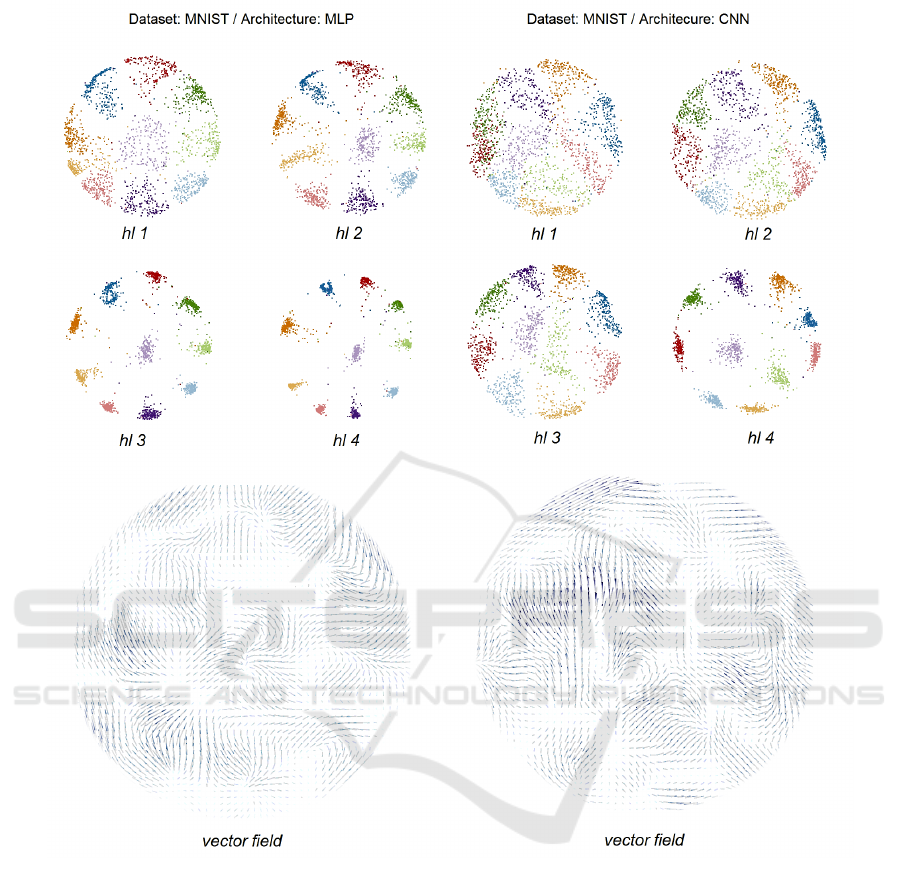
Figure 4: Hidden layer activation projections for the MNIST dataset on MLP(left) and CNN(right), with the obtained vector
fields. The upper area shows the projections of the 4 hidden layers of the fully trained MLP and 4 sampled hidden layers from
the fully trained CNN. While both networks are capable of achieving quite an amount of segmentation on the first layer, the
MLP achieves separation much faster, since the data is pretty much already shown in clusters in the projection of the second
sampled hidden layer. The fact that the vector fields are so muted shows that there is little extra knowledge being generated as
data flows through the layers. The vector field representing the CNN is slightly more intense at the middle, indicating more
movement between layers, which could indicate a class that is taking the network more effort to figure out.
same to those of the original MLP, confirming that
the other layers were in fact unnecessary for this task.
This may indicate, however, that the less immediate
representations of the CNN are more able to adapt and
generalize to different data.
Figure 5 shows the activation projections for the
CIFAR-10 dataset. While the classification results
are worse compared to those of the MNIST, it is in-
stantly clear that there is more action on the vector
fields. There is no smooth expansion: while there is
a clear flow in sections of the field, it is convoluted,
with twists and waves. This means representations are
being formed, but their meaning changes as they are
passed forward through the layers, as instances gen-
erate activations that seem to be oscillating between
being close by or distant in the layer projections. The
intuitive idea is that, in an ideal model, progressing
through layers would mean that instances either get
IVAPP 2020 - 11th International Conference on Information Visualization Theory and Applications
118
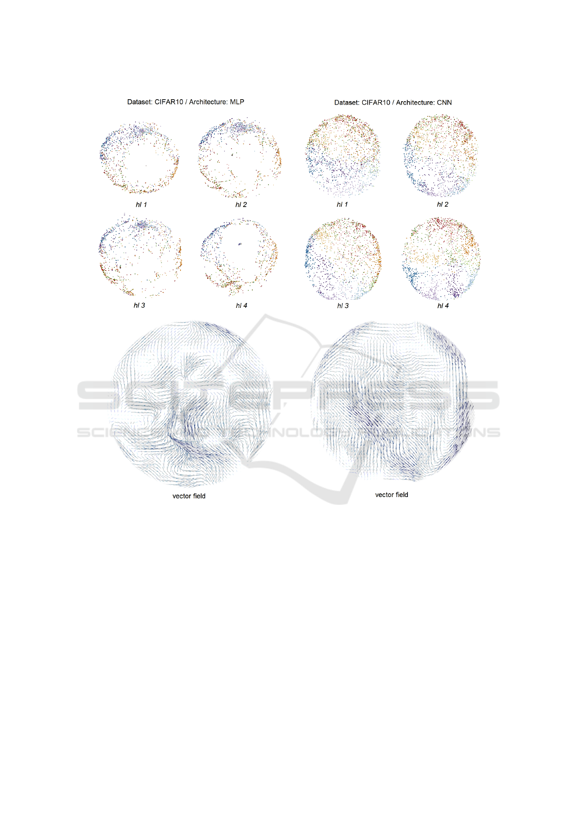
Figure 5: Hidden layer activation projections for the CIFAR10 dataset on MLP(left) and CNN(right), with the obtained vector
fields. The upper area shows projections of 4 hidden layers of the MLP and the 4 sampled layers of the CNN (please see
Experiment Details). The movement happening in these pictures is more twisted and convoluted than before, lacking the
regular expansion we expect to see in ideal results. This movement still means there is information flow through the network,
as more abstract representations are obtained and the relations between objects change, but these representations shift in
meaning and the model seems to fail to make use of the representations it learned.
gradually closer or further apart. That does not hap-
pen here, especially in the MLP model. The CNN
gets to a point where it is possible to see class sepa-
ration (colored zones in the last projections) match-
ing its 75% accuracy value, and this is highlighted
by a smoother vector field. This experiment shows
cases where representations are being formed despite
poor classification results. Going back to the data, it is
possible to search for trajectories most responsible for
defining the vector fields in a certain place (i.e. low
dissimilarity to the vector field, high velocity) and see
which data objects were responsible for that strain of
knowledge in particular, or even identifying trajecto-
ries that are outliers and don’t quite match the approx-
imated vector field.
5 LIMITATIONS
The work described in this paper has certain limita-
tions: one of them is the fact that our projections are
Visualizing Learning Space in Neural Network Hidden Layers
119

forced to be aligned; the visual learning space can
generate distortions in the projected data, as a result of
the matching process between different projections.
As an optimization technique, the method employed
to generate the projections also has random factors,
that need to be accounted for if different sequences of
projections are to be compared as the resulting vector
fields can vary. Additionally, a single vector field may
not be enough to display subtleties of some networks.
There is the possibility of generating a visualization
from multiple vector fields, in order to estimate and
explore more complex visual learning spaces.
6 CONCLUSION
In this paper, we presented a new approach for
projection-based ANN hidden layer visualization that
uses different techniques to provide insights on how
knowledge is generated in a DNN through training
and how abstract representations are formed between
layers. Our focus was to a) adopt a flow-based model
to represent a transition space between projections to
remove point-based clutter and b) present a projection
system capable of holding an aligned view for several
projections, a limitation found in most t-SNE based
techniques. Our approach has other useful character-
istics, namely the ability to compare different data and
to align them using a common feature (e.g., compar-
ing the results of different models applied over the
same objects, or how different parts of a same system
process data) and the generation of a space that tie
different projections together, that may support other
visualization aids in the future. Using this visualiza-
tion, we performed experiments that aim to show how
they can be used to generate knowledge. Our analysis
was able to go further in certain aspects of the training
process of neural networks, attempting to explain sub-
tle aspects of how knowledge is generated in a DNN
system. There are many future research directions re-
garding the work depicted in this paper: as an intro-
ductory study using these methods, the network archi-
tectures used and experiments conducted are the ones
commonly depicted in literature, and more complex
systems and datasets should provide other interesting
analysis opportunities. Additionally, the learning pro-
jection space and vector fields as defined in this paper
assume data from a sequential nature, but there is no
hard restriction limiting them to this type of data.
ACKNOWLEDGMENTS
We would like to thank CAPES and FAPESP
(2017/08817-7, 2015/08118-6) for the financial sup-
port.
REFERENCES
Babiker, H. K. B. and Goebel, R. (2017). An intro-
duction to deep visual explanation. arXiv preprint
arXiv:1711.09482.
Donahue, J., Jia, Y., Vinyals, O., Hoffman, J., Zhang, N.,
Tzeng, E., and Darrell, T. (2014). Decaf: A deep con-
volutional activation feature for generic visual recog-
nition. In International conference on machine learn-
ing, pages 647–655.
Erhan, D., Bengio, Y., Courville, A., and Vincent, P. (2009).
Visualizing higher-layer features of a deep network.
University of Montreal, 1341(3):1.
Ferreira, N., Klosowski, J. T., Scheidegger, C. E., and Silva,
C. T. (2013). Vector field k-means: Clustering trajec-
tories by fitting multiple vector fields. In Computer
Graphics Forum, volume 32, pages 201–210. Wiley
Online Library.
Hamel, P. and Eck, D. (2010). Learning features from mu-
sic audio with deep belief networks. In ISMIR, vol-
ume 10, pages 339–344. Utrecht, The Netherlands.
Hilasaca, G. and Paulovich, F. (2019). Visual feature fusion
and its application to support unsupervised clustering
tasks. arXiv preprint arXiv:1901.05556.
Hohman, F. M., Kahng, M., Pienta, R., and Chau, D. H.
(2018). Visual analytics in deep learning: An interrog-
ative survey for the next frontiers. IEEE Transactions
on Visualization and Computer Graphics.
Joia, P., Coimbra, D., Cuminato, J. A., Paulovich, F. V., and
Nonato, L. G. (2011). Local affine multidimensional
projection. IEEE Transactions on Visualization and
Computer Graphics, 17(12):2563–2571.
Kahng, M., Andrews, P. Y., Kalro, A., and Chau, D. H. P.
(2018). A cti v is: Visual exploration of industry-scale
deep neural network models. IEEE transactions on
visualization and computer graphics, 24(1):88–97.
LeCun, Y., Bengio, Y., and Hinton, G. (2015). Deep learn-
ing. nature, 521(7553):436.
Liu, M., Shi, J., Li, Z., Li, C., Zhu, J., and Liu, S. (2017).
Towards better analysis of deep convolutional neu-
ral networks. IEEE transactions on visualization and
computer graphics, 23(1):91–100.
Mahendran, A. and Vedaldi, A. (2015). Understanding deep
image representations by inverting them. In Proceed-
ings of the IEEE conference on computer vision and
pattern recognition, pages 5188–5196.
Mahendran, A. and Vedaldi, A. (2016). Visualizing
deep convolutional neural networks using natural pre-
images. International Journal of Computer Vision,
120(3):233–255.
IVAPP 2020 - 11th International Conference on Information Visualization Theory and Applications
120

McInnes, L., Healy, J., and Melville, J. (2018). Umap: Uni-
form manifold approximation and projection for di-
mension reduction. arXiv preprint arXiv:1802.03426.
Mohamed, A.-r., Hinton, G., and Penn, G. (2012). Under-
standing how deep belief networks perform acoustic
modelling. neural networks, pages 6–9.
Nonato, L. G. and Aupetit, M. (2018). Multidimensional
projection for visual analytics: Linking techniques
with distortions, tasks, and layout enrichment. IEEE
Transactions on Visualization and Computer Graph-
ics, pages 1–1.
Pezzotti, N., H
¨
ollt, T., Van Gemert, J., Lelieveldt, B. P.,
Eisemann, E., and Vilanova, A. (2018). Deepeyes:
Progressive visual analytics for designing deep neu-
ral networks. IEEE transactions on visualization and
computer graphics, 24(1):98–108.
Rauber, P. E., Fadel, S. G., Falcao, A. X., and Telea, A. C.
(2017). Visualizing the hidden activity of artificial
neural networks. IEEE transactions on visualization
and computer graphics, 23(1):101–110.
Rauber, P. E., Falc
˜
ao, A. X., and Telea, A. C. (2016). Vi-
sualizing time-dependent data using dynamic t-sne. In
Proceedings of the Eurographics/IEEE VGTC Confer-
ence on Visualization: Short Papers, pages 73–77. Eu-
rographics Association.
Scherer, D., M
¨
uller, A., and Behnke, S. (2010). Evaluation
of pooling operations in convolutional architectures
for object recognition. In International conference on
artificial neural networks, pages 92–101. Springer.
Simonyan, K., Vedaldi, A., and Zisserman, A. (2013).
Deep inside convolutional networks: Visualising im-
age classification models and saliency maps. arXiv
preprint arXiv:1312.6034.
Srivastava, N., Hinton, G., Krizhevsky, A., Sutskever, I.,
and Salakhutdinov, R. (2014). Dropout: A simple way
to prevent neural networks from overfitting. The Jour-
nal of Machine Learning Research, 15(1):1929–1958.
Szegedy, C., Liu, W., Jia, Y., Sermanet, P., Reed, S.,
Anguelov, D., Erhan, D., Vanhoucke, V., and Rabi-
novich, A. (2015). Going deeper with convolutions.
In Proceedings of the IEEE conference on computer
vision and pattern recognition, pages 1–9.
Van Der Maaten, L. and Hinton, G. (2008). Visualizing
high-dimensional data using t-sne. journal of machine
learning research. J Mach Learn Res, 9:26.
Wattenberg, M., Vi
´
egas, F., and Johnson, I. (2016). How to
use t-sne effectively. Distill, 1(10):e2.
Yosinski, J., Clune, J., Nguyen, A., Fuchs, T., and Lipson,
H. (2015). Understanding neural networks through
deep visualization. arXiv preprint arXiv:1506.06579.
Zeiler, M. D. and Fergus, R. (2014). Visualizing and under-
standing convolutional networks. In European confer-
ence on computer vision, pages 818–833. Springer.
Zintgraf, L. M., Cohen, T. S., Adel, T., and Welling,
M. (2017). Visualizing deep neural network deci-
sions: Prediction difference analysis. arXiv preprint
arXiv:1702.04595.
Visualizing Learning Space in Neural Network Hidden Layers
121
