
Defect Detection using Deep Learning from Minimal Annotations
Manpreet Singh Minhas
a
and John Zelek
Department of Systems Design Engineering, University of Waterloo, Waterloo, Ontario, Canada
Keywords:
Defect Detection, CNNs, Transfer Learning, Deep Learning.
Abstract:
Visual defect assessment is an important task for infrastructure asset monitoring to detect faults (e.g., road
distresses, bridge cracks, etc) for recognizing and tracking the distress. This is essential to make a decision
on the best course of action, whether that be a minor or major repair or the status quo. Typically a lot of this
surveillance and annotation is done by human operators. Until now, visual defect assessment has been carried
out manually because of the challenging nature of the task. However, the manual inspection method has several
drawbacks, such as training time and cost, human bias and subjectivity, among others. As a result, automation in
visual defect detection has attracted a lot of attention. Deep learning approaches are encouraging the automation
of this detection activity. The actual perceptual surveillance can be conducted with camera-equipped land
vehicles or drones. The automatic defect detection task can be formulated as the problem of anomaly detection
in which samples that deviate from the normal or defect-free ones need to be identified. Recently, Convolutional
Neural Networks (CNNs) have shown tremendous potential in image-related tasks and have outperformed the
traditional hand-crafted feature-based methods. But, CNNs require a large number of labelled data, which
is virtually unavailable for all the practical applications and is a major drawback. This paper proposes the
application of network-based transfer learning using CNNs for the task of visual defect detection that overcomes
the challenge of training from a limited number of samples. Results obtained show that the proposed method
achieves high performance from limited data samples with average F1 score and AUROC values of 0.8914 and
0.9766 respectively. The number of training defect samples were as low as 20 images for the Fray category of
the Magnetic Tile defect data-set.
1 INTRODUCTION
Inspection of surfaces, products, infrastructure such
as roadways, buildings, railways, etc. all involve the
detection of defects and is primarily done for qual-
ity control or assessment and maintenance planning
purposes. In manufacturing, the purpose is to verify
that the product is defect free before installation in the
next level of assembly or for the final distribution of
the product to the customers. While in infrastructure
asset management, defects need to be monitored for
planning maintenance and repairs. Even today, manual
human inspection remains the norm across different
industries. It relies on the basic premise that the sur-
face defects are salient and visually different from the
defect-free surface. This not only makes the process
highly subjective, and susceptible to the human biases
but also prone to errors. The errors in the inspection
process usually have acute consequences such as in-
jury, fatality, loss of expensive equipment, scrapped
a
https://orcid.org/0000-0003-3425-6533
items, rework, or failure to procure repeat business.
Inspection errors can be attributed to the task, environ-
mental, individual, organizational, and social factors
(See et al., 2017). Specifically, individual factors such
as age, visual acuity, scanning strategy, experience
and training impact the errors caused during the man-
ual inspection process. Because of these challenges,
automation of defect detection has been a topic of re-
search across different application areas such as steel
surfaces (Sun et al., 2018), pavements (Ai et al., 2018),
rail tracks (Yu et al., 2019) and fabric (Kumar, 2008).
Even though automatic defect detection has a lot of
potential benefits, it also has its associated challenges.
One of the major ones is that the appearance of defects
varies even within the same inspection task in terms
of shape, size, color, geometry, etc. Also, environ-
mental factors such as changing lighting conditions
and extreme weather add to the detection complexity.
The traditional automation methods have relied on the
computation of a set of hand-crafted textural features
which are then used to train some type of classifier
e.g. SVM. Few examples of these engineered features
506
Minhas, M. and Zelek, J.
Defect Detection using Deep Learning from Minimal Annotations.
DOI: 10.5220/0009168005060513
In Proceedings of the 15th International Joint Conference on Computer Vision, Imaging and Computer Graphics Theory and Applications (VISIGRAPP 2020) - Volume 4: VISAPP, pages
506-513
ISBN: 978-989-758-402-2; ISSN: 2184-4321
Copyright
c
2022 by SCITEPRESS – Science and Technology Publications, Lda. All rights reserved

include Gabor filters (Kumar and Pang, 2002), Fourier
transform (Chi-Ho Chan and Pang, 2000), Wavelet
transform (Serdaroglu et al., 2006) and second-order
statistics derived from spatial gray-level co-occurrence
matrices (Tsai and Huang, 2003). These features suf-
fer from the following drawbacks. They are extremely
difficult to develop and require domain expertise. Also,
they do not generalize i.e. features developed for one
defect cannot be used for other defect detection tasks
without a drastic degradation in the detection perfor-
mance.
In recent years, deep learning approaches and par-
ticularly Convolutional Neural Networks (CNNs) have
outperformed all the traditional hand-crafted feature
based methods in almost all the computer vision tasks.
As a result, there has been a growing interest in au-
tomation of defect detection using deep learning. For
example CNNs were used for rail surface defect clas-
sification (Faghih-Roohi et al., 2016) and steel de-
fect classification (Masci et al., 2012). Although deep
learning methods achieve great performance, they have
the following challenges. Deep learning techniques
require large amounts of labelled training data. But in
real world applications getting labelled training data
is extremely difficult and expensive. Since the occur-
rences of defected examples are very sparse, getting
large amounts of defected instances for training is vir-
tually impossible. As a result training deep neural
networks from scratch for defect detection is difficult
if not impossible.
Transfer Learning is a technique that is used in
practice to tackle this challenge. The goal of trans-
fer learning is to improve learning in a target task
by leveraging knowledge from a source task (Torrey
and Shavlik, 2009). Deep transfer learning can be
broadly classified into four categories: instance-based
deep transfer learning, mapping-based deep transfer
learning, network-based deep transfer learning, and
adversarial based deep transfer learning. Out of these
types, network-based deep transfer learning is most
widely used in practical applications. It refers to the
reuse of a partial network pre-trained for a source do-
main, including its network structure and connection
parameters and transferring it to be a part of deep
neural network which used for a target domain (Tan
et al., 2018). The source network is thought of as
consisting of two sub-networks: (1) Feature extrac-
tor sub-network and (2) Classification sub-network.
The target network is constructed using the source
network with some modifications and trained on the
target dataset for the intended task. The network based
transfer learning approach is shown in Figure 1.
A growing body of literature has examined the use
of transfer learning for different classification tasks.
Kensert et al. applied transfer learning for classifying
cellular morphological changes and explored differ-
ent CNN architectures (Kensert et al., 2019). The
ResNet50 architecture achieving the highest accuracy
of 97.1%. They observed that the models were able to
distinguish the different cell phenotypes despite a lim-
ited quantity of labelled data. In another study, Feng et
al. (Feng et al., 2019) used transfer learning for struc-
tural damage detection. The Inception-v3 architecture
obtained an average accuracy of 96.8% using transfer
learning and outperformed the SVM method which
had an accuracy of 61.2%. Although transfer learning
for classification has been explored for specific appli-
cations, an extensive exploration of anomaly detection
using transfer learning comparing the performance of
the state-of-the-art CNN architectures on different de-
fect detection tasks is missing in the literature. In this
research, we uniquely use the output value from the
neuron responsible for the anomalous samples as the
anomaly score value. And the approach was tested on
three different CNN architectures and four challenging
data-sets. Unlike the current work on defect detection
using transfer learning, we use the AUROC metric
for evaluating the model performance, because it is a
robust and more accurate measure of the separation
capability than just the classification accuracy.
2 RELATED WORK
Automated defect detection is a difficult task and has
a lot of challenges such as complex textures, varying
lighting conditions, different defect shapes, sizes, etc.
Even noise can be different from the normal texture but
should not be classified as a defect. In all real-world
applications, an extremely limited number of anoma-
lous (defective) samples are available. This makes
training any learning based approach difficult. Tradi-
tional methods of defect detection have relied on the
extraction of engineered features specially developed
for particular tasks, which are then fed into a classifier
such as an SVM to make the final detection. However,
these hand-crafted features not only do not generalize
but also are difficult and costly to develop since these
require specific domain knowledge and expertise.
With the recent advances in deep learning, Con-
volutional Neural Networks have outperformed the
traditional methods in almost all the computer vision
related tasks. There have been several studies that
compare deep learning with traditional methods such
as (Hssayeni et al., 2017), (Marnissi et al., 2019), and
(Pogorelov et al., 2018). One finding that is concurrent
with almost all the studies is that the learned features
are better than the non-learned features. Network-
Defect Detection using Deep Learning from Minimal Annotations
507

Domain
A
Source
Feature extractor
Subnetwork
Source
Classification
Subnetwork
Task A
Domain
B
Target
Feature extractor
Subnetwork
Target
Classification
Subnetwork
Task B
Backpropagation
Transfer
Learning
Frozen
Network A
Network B
Figure 1: Illustration of a network-based deep transfer learning from a source domain A and task A to target domain B and task
B. The Network A is trained on a large training dataset and is called the pre-trained network. Network B is constructed by
using parts of Network A followed by a new softmax classification network. Finally, the resulting network B is initialized with
the pre-trained weights and trained using backpropagation on the target dataset.
based transfer learning is a practical technique that
allows the tweaking of the pre-trained (learned) mod-
els for some specific target tasks. And this process can
be done from a limited amount of data.
In one study (Perez et al., 2019), the authors ex-
plored the use of convolutional neural networks for
detecting building defects that is required for effective
management of asset portfolios and improving busi-
ness performance. They used network-based transfer
learning on a VGG-16 network pre-trained on the Ima-
geNet dataset. Also, they approached the problem as a
multi-class classification problem rather than anomaly
detection. The final layer was replaced to have 4 output
neurons and only the last layer weights were updated
during the training. Image augmentation in the form
of rescaling, rotation, etc. was applied. Their approach
achieved a testing accuracy of 87.50%.
Mittel and Kerber (Mittel and Kerber, 2019) ap-
plied vision-based crack detection using transfer learn-
ing in the metal forming process. They also ap-
proached the crack detection as a classification prob-
lem. In their experiments, GoogLeNet outperformed
AlexNet by achieving an F1-score of 0.835. Transfer
learning along with model ensembling was explored
in (Zhang et al., 2019) for weld defect detection and
image augmentation was done using Wasserstein Gen-
erative Adversarial Network. The approach led to
good results with average accuracy of 98% on the de-
fect classes. CNNs were used as fixed feature extractor
followed by training different classifiers for pavement
distress detection in (Gopalakrishnan et al., 2017). In
their experiments, a single layer neural network clas-
sifier trained on features extracted from VGG16 pre-
trained on ImageNet achieved the best performance.
All the existing approaches tackle the defect detec-
tion problem as a single or multi-class classification
problem. The class category is selected by choosing
the one with the highest score. We hypothesize that for-
mulating defect detection as anomaly detection would
lead to better separation capability of the classifier. As-
signing an anomaly score to every image that is the
output value from the neuron responsible for detecting
the anomalous class can give better control over the
classification. While the F1 score is a great metric for
evaluating classification performance, these values can
change depending on the choice of threshold. There-
fore, in this research, we use the AUROC metric (sub-
section 4.4) for evaluating the detector performance
which takes into account all the thresholds. The rest of
the paper is organized as methodology, experiments,
results, and conclusion.
3 METHODOLOGY
The methodology followed in this paper for defect
detection is described by the following steps.
1. Source Model Selection:
A source CNN model
trained on a source data-set for the classification
VISAPP 2020 - 15th International Conference on Computer Vision Theory and Applications
508

task is selected for the network-based transfer
learning. For example, DenseNet161 trained on
the ImageNet data-set.
2. Source Model Modification:
The source model
is then modified by the replacement of the last fully
connected layer with a new layer having two output
neurons. Softmax activation is applied to the layer
to convert the neuron outputs into probabilities.
After this step, the network is ready to be trained
for defect detection.
3. Target Model Transfer Learning:
This step in-
volves the training of the modified neural network
on the target data-set. Two strategies can be used:
(a) Fixed Feature Extractor:
It has been shown
that deep learning models are good at extracting
general features that are better than the tradi-
tional hand-crafted features for classification. In
this case, all the pre-trained network parame-
ter weight values are frozen during training (i.e.
these perimeters won’t be updated during the
optimization process). Only the final fully con-
nected softmax layer weights are learnt during
the training stage.
(b) Full Network Fine Tuning:
In this method, ei-
ther parameters of the entire network or that of
the last
n
layers (parameters frozen for the ini-
tial layers) are updated along with the softmax
classifier during the optimization or training pro-
cedure. A lower learning rate is used because
the pre-trained weights are good and don’t need
to be changed too fast and too much.
4 EXPERIMENTS
In this section, the overall experimental setup includ-
ing the data-sets, CNN architectures, implementation,
training, and evaluation criteria are explained.
4.1 Data-sets
The data-sets used for the experiments are as follows.
1. The German Asphalt Pavement Distress
(GAPs) v2 Data-set:
(Stricker et al., 2019) is
a high quality data-set for pavement distress
detection with damage classes as cracks, potholes,
inlaid patches, applied patches, open joints and
bleeding. The v2 of the data-set has a 50k subset
available for deep learning approaches. It contains
30k normal patches and 20k patches with defects
with a patch size of
256 × 256
for the training set.
And for the testing set there are 6k normal patches
and 4k patches with defects.
2. DAGM Data-set:
(Matthias Wieler, 2007) is a
synthetic data-set for weakly supervised learning
for industrial optical inspection. The data-set con-
tains ten classes of artificially generated textures
with anomalies. For this study, the Class 1 hav-
ing the smudge defect was selected, since it pre-
sented with the maximum intra-class variance of
the background texture. It (hereafter referred to as
DAGMC1) contains
150
images with one defect
per image and 1000 defect free images.
3. Magnetic Tile Defects Data-set:
(Huang et al.,
2018) contains images of magnetic tiles collected
under varying lighting conditions. Magnetic tiles
are used in engines for providing constant mag-
netic potential. There are five different defect types
available namely Blowhole, Crack, Fray, Break
and Uneven. In the experiments in addition to test-
ing the individual defect classes, an MT Defect
category consisting of all the defect types was also
created and considered.
4. Concrete Crack Data-set:
(Fan et al., 2019) con-
tains images of concrete with two classes namely
positive (with the crack defect) and negative (with-
out crack). There are
20, 000 277 × 277
color im-
ages for each class. Images have variance in terms
of surface finish and illumination conditions which
makes the data-set challenging.
4.2 CNN Architectures
The following architectures were selected for conduct-
ing the experiments. Within each category, the model
configuration which achieved the lowest error on the
ImageNet data-set was selected.
1. DenseNet:
Densely Connected Convolutional Net-
works (Huang et al., 2017) (DenseNets) introduced
the concept of inputs from every preceding layer
in the dense blocks. Every layer is connected to
every other layer in a feed-forward fashion so that
the network with L layers has
L(L+1)
2
direct con-
nections. The DenseNet-161 architecture was used
as the source network for the experiments.
2. ResNet:
Deep Residual Networks (He et al., 2016)
introduced the concept of identity shortcut connec-
tions that skip one or more layers. These were
introduced in 2015 by Kaiming He. et.al. and
bagged
1
st
place in the ILSVRC 2015 classifica-
tion competition . ResNet-152 architecture is used
for the experiments.
3. VGGNet:
VGGnet was invented by the Visual
Geometry Group from the University of Oxford.
It introduced the use of successive layers of
3 × 3
Defect Detection using Deep Learning from Minimal Annotations
509

Network Pretrained on
ImageNet with the
Fully Connected Layer
Disconnected
New Fully
Connected layer
with 2 output
classes and softmax
activation
Input
Image
Output
Vector
(2x1)
One Hot
Encoded
Label
(2x1)
Cross Entropy
Loss
Update network parameters
with low learning rate
Figure 2: Defect Detection using network-based transfer learning. A model pre-trained on some source data-set (e.g. ImageNet)
is selected as the base network. The final layers of the network are modified to have two output classes, after which the softmax
activation is applied to convert the neuron outputs into probabilities. The network is then trained on the target data-set with a
much smaller learning rate (e.g.
10
−4
) to adapt it to the new data-set. The output from the anomaly class neuron is then used as
an anomaly score for the sample. A high value indicates that the network is confident that the sample is anomalous.
filters instead of large-size filters such as
11 × 11
and
7 ×7
. VGG19 was chosen for the experiments.
4.3 Implementation
PyTorch (Paszke et al., 2017) version 1.3 was used
for conducting all the experiments. Publicly available
implementations of the selected models were used
from the torchvision package version 0.2.2. Model
weights pre-trained on ImageNet data-set available in
the PyTorch model zoo were used for the experiments.
Adam (Kingma and Ba, 2014) optimizer with default
settings was used. The learning rate was set to
10
−4
.
All the experiments were conducted for 25 epochs.
The input images were resized to
224 ×224 × 3
before
feeding to the network because of the fully connected
layers. The prediction output from the anomaly/defect
neuron was used as the anomaly score and also for
performing the classification. The loss function used
was CrossEntropy which is defined as follows.
H = −
1
n
n
∑
i=1
[y
i
log( ˆy
i
) + (1 − y
i
)log(1 − ˆy
i
)] (1)
where H is the Cross Entropy,
y
i
is the label and
ˆy
i
is
the prediction for the i
th
pixel.
4.4 Evaluation Metrics
To evaluate the quantitative performance of the mod-
els, two metrics were selected. The first metric was
the area under curve (AUC) measurement of the re-
ceiver operating characteristics (ROC) (Ling et al.,
2003). AUC or AUROC is a reliable measure of the
degree or measure of the separability of any binary
classifier (binary segmentation masks in this case). It
provides an aggregate measure of the model’s perfor-
mance across all possible classification thresholds. An
excellent model has AUROC value near to the one and
it means that the classifier is virtually agnostic to the
choice of a particular threshold. The second metric
used for the assessment was the F1 score. It is defined
as the harmonic mean of precision and recall and is
given by the Equation 2. F1 score reaches its best
value at one and the worst score at zero. It is a robust
choice for classification tasks since it takes both the
false positives and false negatives into account.
F = 2 ×
P × R
P + R
(2)
where F is the F1 score, P is the precision and R is the
recall.
VISAPP 2020 - 15th International Conference on Computer Vision Theory and Applications
510

5 RESULTS
Figure 3 summarises the results of all the experiments
conducted for the various data-sets and CNN architec-
ture configurations. Figures 3 (a), (b) and (c) show
the AUROC and F1 Score values for the Fixed Feature
Extractor and Full Network Fine Tuning experiments
for DenseNet161, ResNet152 and Vgg19 respectively.
The values shown are for the best model per architec-
ture and data-set based on the lowest validation loss. It
is important to note that for calculating the F1 scores a
threshold value of 0.5 was used since that is the mean
value of the output range of the neuron with softmax
activation applied to it. The F1 score value will vary
depending on the choice of threshold. But the AUROC
score takes into account all the possible threshold val-
ues in its calculation. One clear observation from all
the experiments is that on average, across all the data-
set and CNN architecture configurations Full Network
Fine Tuning worked better than the Fixed Feature Ex-
tractor approach. Table 1 shows comparison between
the two. This showed that the initial layers which are
often attributed to being good at extracting general
features, also need to be trained while performing the
network-based transfer learning. Fine tuning the net-
work weights with a lower learning rate in comparison
to the learning rate used during the training on the
source data-set leads to weights that better optimize
the cost function for the target task and data-set.
On average across all the data-sets, using the Full
Network Fine Tuning approach the Vgg19 architec-
ture performed the best with F1 Score and AUROC
values of 0.8914 and 0.9766 respectively. In the fixed
feature extractor approach Vgg19 performed the best
on an average based on the AUROC value. While the
DenseNet161 performed the best based on F1 score.
The highest average performance gap between the two
approaches was observed in the ResNet152 model,
with a difference of 97% and 44% for F1 score and AU-
ROC value respectively. And the lowest gap with re-
spect to the F1 score and AUROC value was obaserved
for DenseNet161 and Vgg19 at 83% and 28% respec-
tively. DAGMC1 was the only synthetic data-set in
the experiments and as expected all the three archi-
tectures are perfectly able to separate the defects or
anomalies from the normal samples. On the extremely
challenging GAPSv2 data-set DenseNet161 performed
the best with F1 Score and AUROC values of 0.9882
and 0.9979 respectively. ConcreteCrack data-set is the
only data-set on which on average the fixed feature
extractor approach performed better than the full net-
work fine-tuning. However, the performance gap was
marginal in comparison to other data-sets. It was 2%
for the F1 Score and 4% for the AUROC value. On the
magnetic tile dataset (data-sets with the prefix MT) as
expected average of the best models trained for single
defect category outperformed the best model trained
on the mixture of all the defects. The improvement
for F1 Score and AUROC values was that of 6% and
4% respectively. Another thing to note is that the out-
put of the anomaly or defect neuron being used as an
anomaly score worked well which is in concurrence
with our hypothesis. It resulted in a very high separat-
ing power of the networks between the anomalous and
normal samples. This is evident from the impressive
average AUROC value of 0.9766 as mentioned earlier
in this section.
Table 1: Comparison of Full Network and Fixed Feature
extraction approach. The values shown are averaged across
all the data-sets. As can be seen, the Full Network approach
clearly outperforms the Fixed Feature approach across the
three architectures.
Model
Full Network Fixed Feature
F1 Score AUROC F1 Score AUROC
DenseNet161 0.8477 0.9087 0.4639 0.6874
ResNet152 0.8259 0.9570 0.4183 0.6631
Vgg19 0.8914 0.9766 0.4543 0.7600
6 CONCLUSION
In this paper, we applied the concept of network-based
transfer learning using CNNs to the task of defect
detection. The approach tackles the challenge of a lim-
ited number of anomalous samples available in real-
world applications. The method achieves impressive
values of 0.8914 and 0.9766 for F1 Score and AUROC
respectively across four challenging data-sets. Within
the network-based transfer learning approach two tech-
niques were tested i.e., Fixed Feature Extraction and
Full Network Fine Tuning. It was found that the full
network fine tuning approach on an average across
all the data-sets tended to work much better than the
fixed feature extraction approach. Additionally, the
use of the output value from the neuron responsible
for the anomaly or defect class as an anomaly score
led to excellent AUROC values indicating the strong
separation power of the CNNs across all the data-sets.
For future work, it would be interesting to see how
the choice of the activation function of the final classi-
fier affects defect detection performance. Additionally,
experiments can be conducted on freezing only a few
selected layers of the model and evaluating the change
in performance. More CNN architectures can be anal-
ysed to see how the choice of architecture affects the
performance for different defect types.
Defect Detection using Deep Learning from Minimal Annotations
511
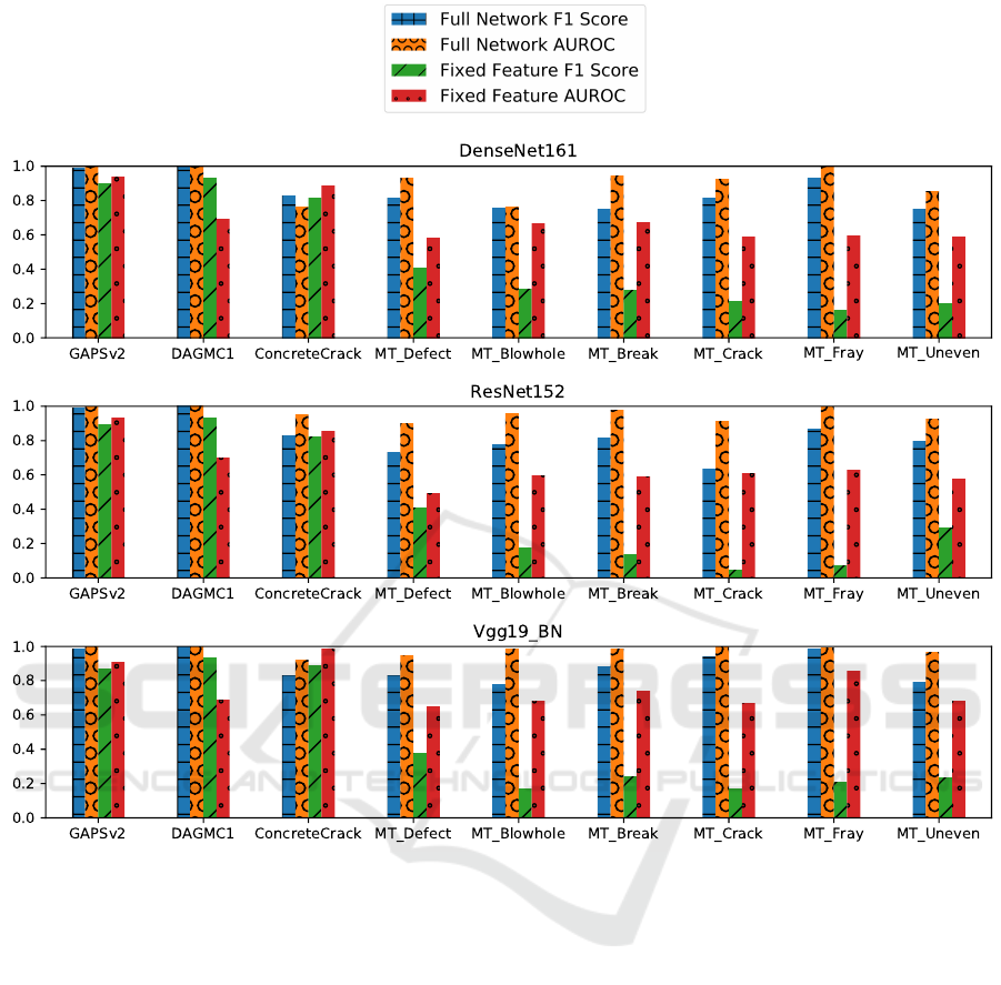
Figure 3: Results of the experiments conducted on all the data-sets and CNN architectures. Figures 3 (a), (b) and (c) show the
AUROC and F1 Score values for the Fixed Feature Extractor and Full Network Fine Tuning experiments for DenseNet161,
ResNet152 and Vgg19 respectively. The values shown are for the best model per architecture and data-set based on the lowest
validation loss. It can be observed across the data-sets and the architectures, that on an average the full network fine tuning
seems to work better than the fixed feature extractor approach. (Best viewed in colour.)
ACKNOWLEDGEMENTS
The authors would like to thank the Ontario Ministry
of Transportation and NSERC (National Science and
Research Council) for providing funds that supported
this research.
REFERENCES
Ai, D., Jiang, G., Siew Kei, L., and Li, C. (2018). Automatic
pixel-level pavement crack detection using information
of multi-scale neighborhoods. IEEE Access, 6:24452–
24463.
Chi-Ho Chan and Pang, G. K. H. (2000). Fabric defect
detection by fourier analysis. IEEE Transactions on
Industry Applications, 36(5):1267–1276.
Faghih-Roohi, S., Hajizadeh, S., Nez, A., Babuska, R., and
De Schutter, B. (2016). Deep convolutional neural
networks for detection of rail surface defects. In 2016
International Joint Conference on Neural Networks
(IJCNN), pages 2584–2589.
Fan, R., Bocus, M. J., Zhu, Y., Jiao, J., Wang, L., Ma, F.,
Cheng, S., and Liu, M. (2019). Road crack detection
using deep convolutional neural network and adaptive
thresholding. 2019 IEEE Intelligent Vehicles Sympo-
sium (IV), pages 474–479.
Feng, C., Zhang, H., Wang, S., Li, Y., Wang, H., and Yan, F.
(2019). Structural damage detection using deep convo-
lutional neural network and transfer learning. KSCE
VISAPP 2020 - 15th International Conference on Computer Vision Theory and Applications
512

Journal of Civil Engineering, 23(10):4493–4502.
Gopalakrishnan, K., Khaitan, S. K., Choudhary, A., and
Agrawal, A. (2017). Deep convolutional neural net-
works with transfer learning for computer vision-based
data-driven pavement distress detection. Construction
and Building Materials, 157:322 – 330.
He, K., Zhang, X., Ren, S., and Sun, J. (2016). Deep residual
learning for image recognition. 2016 IEEE Conference
on Computer Vision and Pattern Recognition (CVPR),
pages 770–778.
Hssayeni, M. D., Saxena, S., Ptucha, R., and Savakis, A.
(2017). Distracted driver detection: Deep learning vs
handcrafted features. Electronic Imaging, 2017(10):20–
26.
Huang, G., Liu, Z., van der Maaten, L., and Weinberger,
K. Q. (2017). Densely connected convolutional net-
works. 2017 IEEE Conference on Computer Vision
and Pattern Recognition (CVPR), pages 2261–2269.
Huang, Y., Qiu, C., and Yuan, K. (2018). Surface defect
saliency of magnetic tile. The Visual Computer.
Kensert, A., Harrison, P. J., and Spjuth, O. (2019). Transfer
learning with deep convolutional neural networks for
classifying cellular morphological changes. SLAS DIS-
COVERY: Advancing Life Sciences R&D, 24(4):466–
475. PMID: 30641024.
Kingma, D. P. and Ba, J. (2014). Adam: A method for
stochastic optimization. CoRR, abs/1412.6980.
Kumar, A. (2008). Computer-vision-based fabric defect
detection: A survey. IEEE Transactions on Industrial
Electronics, 55(1):348–363.
Kumar, A. and Pang, G. K. H. (2002). Defect detection in
textured materials using gabor filters. IEEE Transac-
tions on Industry Applications, 38(2):425–440.
Ling, C. X., Huang, J., and Zhang, H. (2003). Auc: A sta-
tistically consistent and more discriminating measure
than accuracy. In Proceedings of the 18th International
Joint Conference on Artificial Intelligence, IJCAI’03,
pages 519–524, San Francisco, CA, USA. Morgan
Kaufmann Publishers Inc.
Marnissi, M. A., Fradi, H., and Dugelay, J. (2019). On the
discriminative power of learned vs. hand-crafted fea-
tures for crowd density analysis. In 2019 International
Joint Conference on Neural Networks (IJCNN), pages
1–8.
Masci, J., Meier, U., Ciresan, D. C., Schmidhuber, J., and
Fricout, G. (2012). Steel defect classification with
max-pooling convolutional neural networks. The 2012
International Joint Conference on Neural Networks
(IJCNN), pages 1–6.
Matthias Wieler, T. H. (2007). Weakly supervised learning
for industrial optical inspection. https://hci.iwr.uni-
heidelberg.de/node/3616.
Mittel, D. and Kerber, F. (2019). Vision-based crack de-
tection using transfer learning in metal forming pro-
cesses. In 2019 24th IEEE International Conference
on Emerging Technologies and Factory Automation
(ETFA), pages 544–551.
Paszke, A., Gross, S., Chintala, S., Chanan, G., Yang, E.,
DeVito, Z., Lin, Z., Desmaison, A., Antiga, L., and
Lerer, A. (2017). Automatic differentiation in PyTorch.
In NIPS Autodiff Workshop.
Perez, H., Tah, J. H. M., and Mosavi, A. (2019). Deep learn-
ing for detecting building defects using convolutional
neural networks. Sensors, 19(16):3556.
Pogorelov, K., Ostroukhova, O., Petlund, A., Halvorsen, P.,
de Lange, T., Espeland, H. N., Kupka, T., Griwodz, C.,
and Riegler, M. (2018). Deep learning and handcrafted
feature based approaches for automatic detection of
angiectasia. In 2018 IEEE EMBS International Confer-
ence on Biomedical Health Informatics (BHI), pages
365–368.
See, J. E., Drury, C. G., Speed, A., Williams, A., and Kha-
landi, N. (2017). The role of visual inspection in the
21st century. Proceedings of the Human Factors and
Ergonomics Society Annual Meeting, 61(1):262–266.
Serdaroglu, A., Ertuzun, A., and Ercil, A. (2006). Defect
detection in textile fabric images using wavelet trans-
forms and independent component analysis. Pattern
Recognition and Image Analysis, 16(1):61–64.
Stricker, R., Eisenbach, M., Sesselmann, M., Debes, K., and
Gross, H.-M. (2019). Improving visual road condition
assessment by extensive experiments on the extended
gaps dataset. In International Joint Conference on
Neural Networks (IJCNN), pages 1–8.
Sun, X., Gu, J., Tang, S., and Li, J. (2018). Research progress
of visual inspection technology of steel products a
review. Applied Sciences, 8(11).
Tan, C., Sun, F., Kong, T., Zhang, W., Yang, C., and Liu, C.
(2018). A survey on deep transfer learning. In ICANN
2018.
Torrey, L. and Shavlik, J. W. (2009). Transfer learning.
Tsai, D.-M. and Huang, T.-Y. (2003). Automated surface
inspection for statistical textures. Image and Vision
Computing, 21(4):307 – 323.
Yu, H., Li, Q., Tan, Y., Gan, J., Wang, J., Geng, Y., and Jia, L.
(2019). A coarse-to-fine model for rail surface defect
detection. IEEE Transactions on Instrumentation and
Measurement, 68(3):656–666.
Zhang, H., Chen, Z., Zhang, C., Xi, J., and Le, X. (2019).
Weld defect detection based on deep learning method.
In 2019 IEEE 15th International Conference on Au-
tomation Science and Engineering (CASE), pages
1574–1579.
Defect Detection using Deep Learning from Minimal Annotations
513
