Glioma Grade Classiﬁcation via Omics Imaging

Lucia Maddalena

1 a

, Ilaria Granata

1 b

, Ichcha Manipur

, Mario Manzo

2 c

and Mario R. Guarracino

1 d

Inst. for High-Performance Computing and Networking, National Research Council, Via P. Castellino, 111, Naples, Italy

Information Technology Services, University of Naples “L’Orientale”, Via Nuova Marina, 59, Naples, Italy

Keywords:

Glioma Grade Classiﬁcation, Metabolic Networks, Omics Imaging.

Abstract:

Omics imaging is an emerging interdisciplinary ﬁeld concerned with the integration of data collected from

biomedical images and omics experiments. Bringing together information coming from different sources, it

permits to reveal hidden genotype-phenotype relationships, with the aim of better understanding the onset

and progression of many diseases, and identifying new diagnostic and prognostic biomarkers. In this work,

we present an omics imaging approach to the classiﬁcation of different grades of gliomas, which are primary

brain tumors arising from glial cells, as this is of critical clinical importance for making decisions regarding

initial and subsequent treatment strategies. Imaging data come from analyses available in The Cancer Imag-

ing Archive, while omics attributes are extracted by integrating metabolic models with transcriptomic data

available from the Genomic Data Commons portal. We investigate the results of feature selection for the two

types of data separately, as well as for the integrated data, providing hints on the most distinctive ones that

can be exploited as biomarkers for glioma grading. Moreover, we show how the integrated data can provide

additional clinical information as compared to the two types of data separately, leading to higher performance.

We believe our results can be valuable to clinical tests in practice.

1 INTRODUCTION

Gliomas are neuroepithelial tumors affecting glial

cells of the central nervous system (CNS) and are the

most common primary form of brain tumors. The

classiﬁcation and grading of gliomas have evolved

over time, since 1926 until the modern classiﬁca-

tion based on the World Health Organization (WHO)

classiﬁcation of CNS tumors, ﬁrst published in 1979

and then revised several times, most recently in

2016 (Louis et al., 2016). The WHO classiﬁca-

tion system categorizes gliomas from grade I (lowest

grade) to grade IV (highest grade), based on several

morphologic, histological, and molecular attributes.

The differentiation between low-grade gliomas

(LGGs) and high-grade gliomas (HGGs) is critical,

since the prognosis, and thus the therapeutic strategy,

could differ substantially depending on the grade. In-

deed, HGGs are usually treated with surgical resec-

tion, followed by radiation therapy and chemother-

https://orcid.org/0000-0002-0567-4624

https://orcid.org/0000-0002-3450-4667

https://orcid.org/0000-0001-8727-9865

https://orcid.org/0000-0003-2870-8134

apy. If they are misdiagnosed as LGGs, then they

will be treated less effectively (Togao et al., 2016).

A further distinction has to be made in the context

of HGGs, where the last grade, namely GlioBlas-

toma Multiforme (GBM), is the most aggressive dif-

fuse heterogeneous glioma with poor prognosis and

complex treatment, so much to be considered almost

untreatable (Soeda et al., 2015).

The extraction of large amounts of quantitative

features from medical images, often referred to as ra-

diomics (Lambin et al., 2012; Kumar et al., 2012),

has emerged in the last decade as a powerful method-

ology to quantify the characteristics of tumors in a

non-invasive manner, providing imaging biomarkers

for supporting clinical decision-making (Cho et al.,

2018). This approach has been investigated also for

the classiﬁcation of glioma grades (Law et al., 2003;

Zacharaki et al., 2009; Togao et al., 2016; Cho et al.,

2018; Ertosun and Rubin, 2015; Khawaldeh et al.,

2018), where conventional and advanced Magnetic

Resonance Imaging (MRI) techniques are adopted to

extract a variety of imaging features.

With the advent of high-throughput arrays and

Next Generation Sequencing technologies, it is

now possible to integrate information coming from

Maddalena, L., Granata, I., Manipur, I., Manzo, M. and Guarracino, M.

Glioma Grade Classiﬁcation via Omics Imaging.

DOI: 10.5220/0009167700820092

In Proceedings of the 13th International Joint Conference on Biomedical Engineering Systems and Technologies (BIOSTEC 2020) - Volume 2: BIOIMAGING, pages 82-92

ISBN: 978-989-758-398-8; ISSN: 2184-4305

biomedical images with the omics data, i.e., those ob-

tained by the large-scale characterization and quan-

tiﬁcation of molecules present in cells. A new in-

terdisciplinary ﬁeld is emerging, concerned with the

integration of data collected from biomedical images

and omics analyses. Often named imaging genomics

(Hariri and Weinberger, 2003; Jaffe, 2012; Lee et al.,

2017) or radiogenomics (Acharya et al., 2018; Gillies

et al., 2016; Sala et al., 2017), we refer to it as

omics imaging (Antonelli et al., 2019), to better re-

ﬂect the wide variety of omics (genomics, transcrip-

tomics, proteomics, other omics) data that can be ex-

ploited and combined with structural, functional, and

molecular imaging data. Bringing together informa-

tion coming from different sources, it permits to re-

veal hidden genotype-phenotype relationships, with

the aim of better understanding the onset and progres-

sion of various diseases, and identifying new diagnos-

tic and prognostic biomarkers (Ranjbar and Mitchell,

2017).

Several omics imaging studies investigated the re-

lationship between GBM imaging phenotypes, eval-

uated by MR images (Diehn et al., 2008; Zinn

et al., 2011; Beig et al., 2017) or CT images (Jain

et al., 2012), and gene-expression proﬁles, assessed

by cDNA microarray (Diehn et al., 2008; Zinn et al.,

2011; Smedley and Hsu, 2018) or RNA-seq analy-

ses (Beig et al., 2017). Some of them also investigated

the possible predictive value of the omics imaging ap-

proach for the survival of GBM patients (e.g., (Diehn

et al., 2008; Gevaert et al., 2014)). However, to our

knowledge, none of them was devoted to the classiﬁ-

cation of the glioma grades.

In this work, we present an omics imaging ap-

proach to the classiﬁcation of glioma grades. We start

integrating a dataset with both imaging and omics

data for each patient, collecting the data from publicly

available sources. Imaging features extracted by MRI

data come from publicly available analyses (Bakas

et al., 2017a), while, based on previous work (Granata

et al., 2019), we show how to integrate omics vari-

ables to span a new feature space. Finally, we re-

port and analyze results using or not feature selection

and oversampling, empirically proving that the inte-

gration of imaging and omics features, together with

these techniques, can lead to improved performance.

2 MATERIALS AND METHODS

2.1 Data

Omics data come from The Cancer Genome Atlas

(TCGA, tcga-data.nci.nih.gov), a multi-institutional

comprehensive collection of various molecularly

characterized tumor types, whose data are avail-

able through the NCI’s Genomic Data Commons

portal (gdc.cancer.gov). Speciﬁcally, we exploited

FPKM (fragments per kilobase per million reads

mapped) normalized gene counts from RNA sequenc-

ing data of two brain cancer projects, TCGA-GBM

and TCGA-LGG. TCGA-GBM contains data for 161

samples, while TCGA-LGG contains data for 511

samples (see the “O” column in Table 1). For these

Table 1: Number of samples for the Omics dataset (O), the

Imaging dataset (I), and their intersection (OI).

Collection O I OI

TCGA-GBM 161 135 30

TCGA-LGG 511 108 104

Total 672 243 134

data, we extracted features based on a metabolic

model of brain tissue (Agren et al., 2012), down-

loaded from the Metabolic Atlas database (metabol-

icatlas.org). Speciﬁcally, by combining samples

of gene expression data with the tissue-speciﬁc

metabolic model, a weighted directed multigraph for

each sample is obtained (Granata et al., 2019). Its

nodes represent the involved metabolites; the edges

connect interacting metabolites, and their weights are

the expression values of the enzymes catalyzing the

reactions in which the couple of metabolites is in-

volved. The multigraphs are reduced to simple graphs

as in (Granata et al., 2018), by taking the mean of the

expression values for multiple enzymes connecting

two nodes in the same reaction and then summing up

the means of different reactions connecting the couple

of metabolites. This way, each network contains 8458

edges, reduced to 1375 by eliminating edges having

weights common to all samples, used in the follow-

ing as omics features (O). The scheme of the proce-

dure for collecting omics features is reported in Fig.

1 (left).

Imaging data consist of multimodal MRI im-

ages publicly available from The Cancer Imag-

ing Archive (TCIA, cancerimagingarchive.net) (Clark

et al., 2013), where case-linked diagnostic pre-

surgical images are available for a large subset of the

TCGA genomically analyzed cases. Imaging features

are those available in the TCIA archive as analysis re-

sults provided by Bakas et al. (Bakas et al., 2017a;

Bakas et al., 2017b; Bakas et al., 2017c), extracted

from images of the TCGA-GBM and TGCA-LGG

collections. A subset of the available radiological

data was selected by the authors, including those that

refer to pre-operative baseline scans with available

MRI modalities of at least T1-weighted pre-contrast

Glioma Grade Classiﬁcation via Omics Imaging

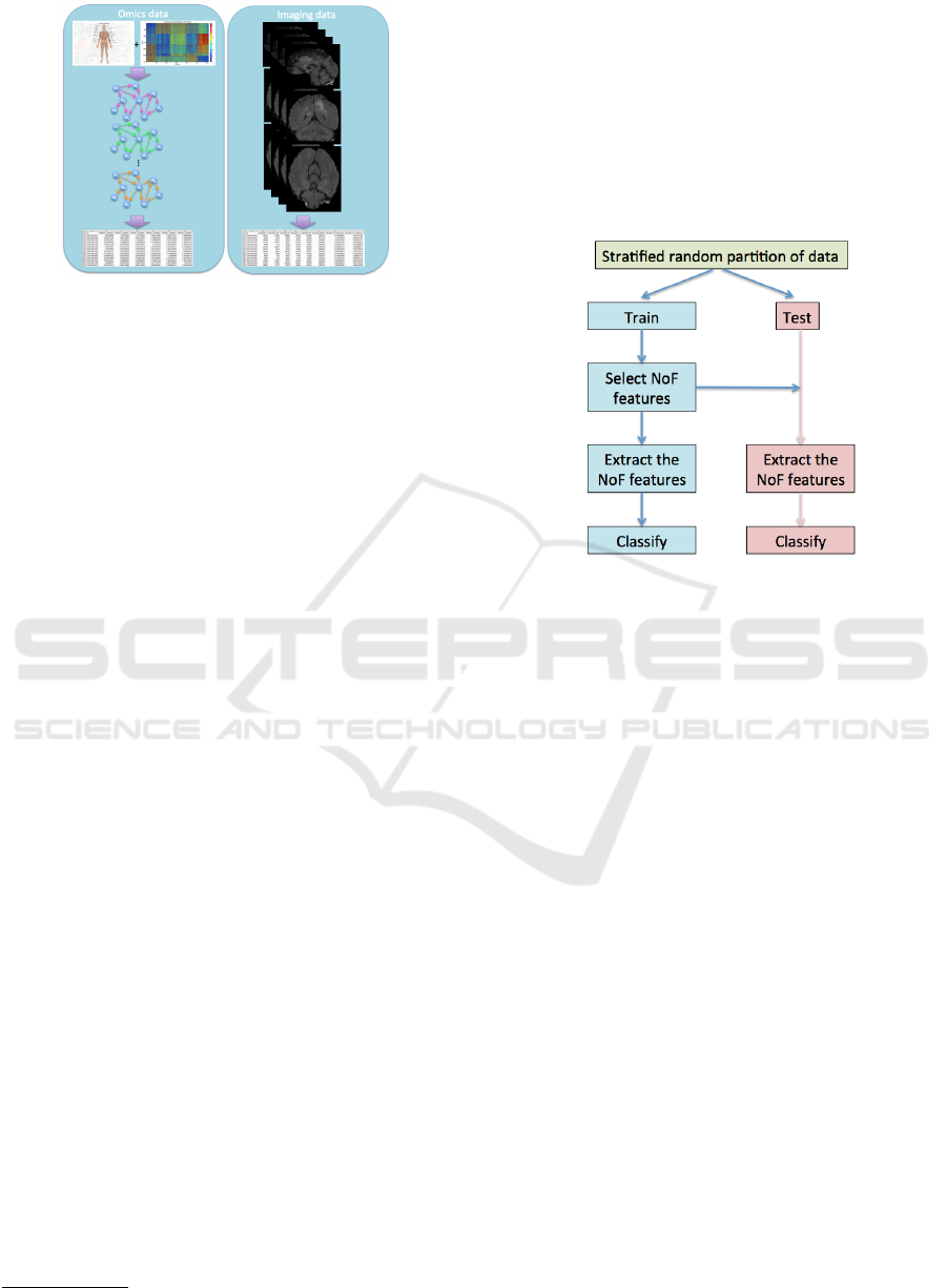
Figure 1: Omics and Imaging data. Omics data (left) are

obtained by the simpliﬁcation of multigraphs constructed

by the metabolic model of brain tissue used for the RNA

sequencing data. Imaging data (right) consist of radiomics

features volumetrically extracted by MRI images.

(T1), T1-weighted post-contrast (T1-Gd), T2, and

T2-FLAIR. After pre-processing and segmentation of

different glioma sub-regions, a panel of more than

700 features was extracted volumetrically by the se-

lected image data. These features provide quantita-

tive information regarding intensity, volumes, mor-

phology, histogram-based, and textural parameters, as

well as spatial information and parameters extracted

from glioma growth models. The features have been

computed by the authors for 135 TCGA-GBM sub-

jects and 108 TGCA-LGG subjects (see “I” column

in Table 1). Among them, those for 102 GBM and 65

LGG samples are publicly available through TCIA,

while the remaining features, used for the MICCAI

Brain Tumor Segmentation 2018 (BraTS 2018)

test

data set, are available upon demand.

Matching the subject IDs of imaging and omics

data, we obtained a total of 30 samples from TCGA-

GBM and 104 samples from TCGA-LGG having both

omics and imaging data (see “OI” column in Table 1).

In the following, the whole sets of omics, imaging,

and omics imaging features for the matched samples

will be denoted as O, I, and OI, respectively.

In case of feature selection (see Sect. 2.2.1), two

integration strategies will be considered: 1) the inte-

grated data consists of the features selected among the

whole OI concatenated set (again referred to as OI),

and 2) the integrated data consists of the concatena-

tion of the two sets of selected omics and imaging

features (referred to as OpI).

2.2 Classiﬁcation Procedure

The procedure adopted for classiﬁcation follows a

typical workﬂow, as reported in Fig. 2. The input

https://www.med.upenn.edu/sbia/brats2018.html

data (either O, I, or OI features) is partitioned into a

training and a testing set containing 66% and 33% of

the samples, respectively. The partitioning is chosen

randomly, taking care to have the same distribution of

samples over classes, both in training and in test set.

The training set is used to determine an optimal subset

of features (see Sect. 2.2.1). This subset is extracted

from both the training and the testing set and used for

classiﬁcation (see Sect. 2.2.2).

Figure 2: Scheme of the classiﬁcation procedure. Data is

partitioned into a training and a testing set. The training

set is used to determine an optimal subset of features. This

subset is extracted from both the training and the testing set

and used for classiﬁcation.

2.2.1 Feature Selection

It is well-known that feature selection is generally a

fundamental step prior to classiﬁcation (Wang et al.,

2016). This is even more compelling in the case of

omics imaging. Indeed, ﬁrst of all, the overall number

of features is in the order of tens of thousand, giving

rise to the well-known curse of dimensionality. The

associated mathematical problem is ill-posed because

the number of variables is generally far larger than

the number of samples. When the number of sam-

ples is low, the features might appear highly corre-

lated. Moreover, the number of features represent-

ing the two types of data is very unbalanced: omics

data are described by tens of thousands of variables,

whereas the imaging variables are usually in the order

of hundreds. This imbalance produces a high proba-

bility of selecting features by chance from the omics

data. Finally, the information-to-noise ratio is differ-

ent in imaging and omics data, which might lead to

overﬁtting classiﬁcation models.

For feature selection, we use SVM-RFE (Guyon

et al., 2002), a wrapper method based on recursive

feature elimination using Support Vector Machines

(SVM) (Vapnik, 1995), that provides a ranked list

BIOIMAGING 2020 - 7th International Conference on Bioimaging

of features ordered according to their relevance. To

choose the optimal number of features to be selected

from a dataset, we perform a k-fold cross-validation

(CV) of a classiﬁcation model (see Sect. 2.2.2)

trained using the ﬁrst NoF sorted features of the train-

ing data and choose the value of NoF that maximizes

the achieved performance across niter iterations of

the process (see Fig. 3). In the experiments, we set

k=5 and niter=10; NoF is searched in the interval

[10,20], experimentally proved to be suitable for all

O, I, and OI data, maximizing the AUC measure.

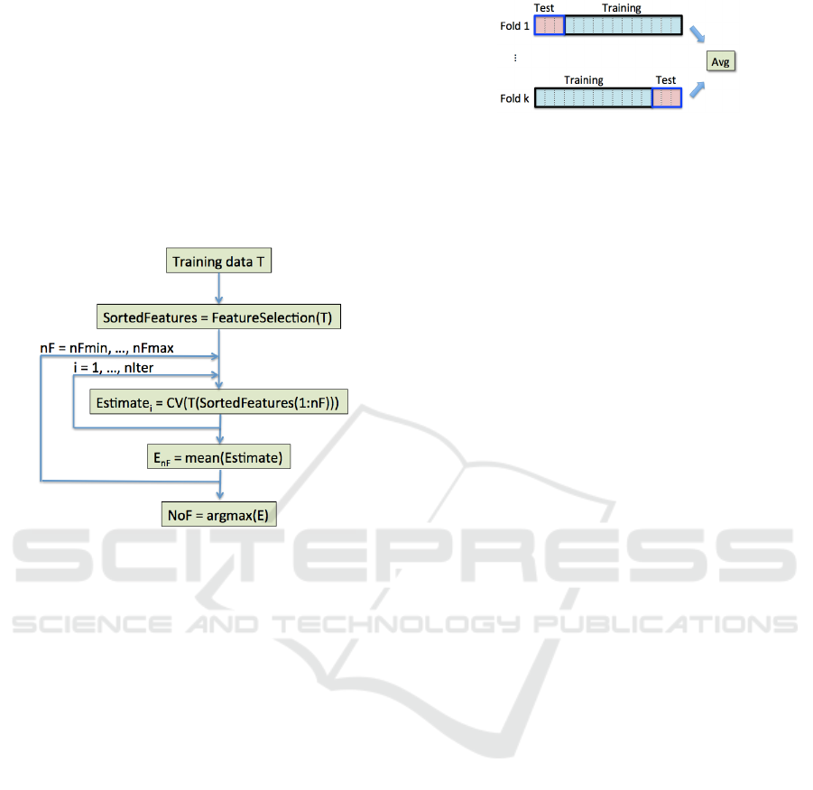
Figure 3: Selection of NoF features. Once features from

the training data are ranked, their optimal number NoF is

chosen as the one that maximizes average performance, es-

timated through CV.

2.2.2 Classiﬁcation

For supervised classiﬁcation, as well as for choos-

ing the optimal number of selected features, several

classiﬁers can be considered. In the experiments, we

report results using the k-Nearest Neighbor classiﬁer

(k=1), deemed to be among the top 10 techniques for

data mining (Wu et al., 2007).

2.2.3 Evaluation

For evaluating the classiﬁcation results, the classiﬁca-

tion procedure of Fig. 2 is repeated a number numIter

of times (in the experiments, numIter is set to 50),

each time randomly permuting the data and validat-

ing the classiﬁcation of the extracted features through

k-fold CV (see Fig. 4). In the experiments, k is set to

5. Overall performance values are obtained as the av-

erage of those obtained at each iteration (i.e., for each

of the partitions).

Figure 4: Scheme of k-fold cross-validation. Data is divided

into k subsets. At each of the k iterations, one subset is

used as the test set and the other k-1 subsets are used as the

training set. The k results are averaged to produce a single

estimation.

2.2.4 Handling Imbalanced Data

Considering a binary classiﬁcation problem, a dataset

is said to be imbalanced if there exists an under-

represented concept (a minority class) when com-

pared to the other (a majority class). The imbalance

ratio (IR), i.e., the ratio of the cardinalities of the ma-

jority and the minority classes, is usually adopted to

establish the imbalance severity. Prediction models

built from imbalanced datasets are often biased to-

wards the majority concept, which is especially crit-

ical when there is a higher cost of misclassifying the

minority examples, as in our case for diagnosing the

highest glioma grade. For recent discussions on han-

dling imbalanced data, see (Peeken et al., 2018; San-

tos et al., 2018; Manzo, 2019). The problem is even

more challenging in the context of omics imaging,

since imaging and omics techniques analyze phenom-

ena that might have intrinsic differences and different

sensitivity levels (Antonelli et al., 2019).

As the IR in our datasets is quite high (IR=3.47),

in our experiments, we adopted the Adaptive syn-

thetic sampling approach for imbalanced learning

(ADASYN) oversampling method (Haibo He et al.,

2008), an extension of Synthetic Minority Over-

sampling Technique (SMOTE) (Chawla et al., 2002)

that synthetically creates new samples of the minority

class via linear interpolation between existing minor-

ity class samples. Those minority samples that are

harder to learn are given greater importance; thus,

they are oversampled more often. Therefore, most of

the new samples lay in the vicinity of the boundary

between the two classes, rather than in the interior of

the minority class.

2.2.5 Cross Validation for Imbalanced Data

In our framework, CV is adopted for both feature se-

lection (see Sect. 2.2.1) and overall evaluation (see

Sect. 2.2.3). It is well known that the joint appli-

cation of CV with oversampling should be handled

with care (Santos et al., 2018). Speciﬁcally, over-

sampling should not be applied to the entire original

Glioma Grade Classiﬁcation via Omics Imaging

data, over which to perform CV and model evaluation,

as this procedure would lead to building biased mod-

els and producing overoptimistic error estimates. In-

stead, oversampling should be applied during CV (see

Fig. 5), only on the training data of each fold, so that

exact or similar replicas of a given pattern produced

by oversampling cannot be found in both the training

and test sets. In our experiments using oversampling,

Figure 5: Scheme of k-fold cross-validation with oversam-

pling. At each step, oversampling (for balancing green and

red classes) is performed only on subsets used for training.

Red samples with * indicate artiﬁcial samples added to the

minority (red) class.

the standard CV (as depicted in Fig. 4) is replaced by

the CV with oversampling sketched in Fig. 5, for both

feature selection and evaluation.

3 RESULTS AND DISCUSSION

3.1 Performance Measures

In our experiments, we consider several performance

metrics, deﬁned in terms of the number of true pos-

itives (TP), true negatives (TN), false positives (FP)

and false negatives (FN)

• Accuracy (Acc): measures the percentage of cor-

rectly classiﬁed examples and is computed as

Acc =

T P + T N

T P + FN + FP + T N

; (1)

• Speciﬁcity (Spec): measures the percentage of

negative examples correctly identiﬁed and is de-

ﬁned as

Spec =

T N

T N + FP

; (2)

• Sensitivity (Sens): also referred to as Recall, it

measures the percentage of positive examples cor-

rectly classiﬁed and is computed as

Sens =

T P

T P + FN

; (3)

• Precision (Prec): corresponds to the percentage

of positive examples correctly classiﬁed, consid-

ering the set of all the examples classiﬁed as pos-

itive, and is deﬁned as

Prec =

T P

T P + FP

; (4)

• F-measure (F

): shows the compromise between

sensitivity and precision, obtained as

= (1 + β

) ·

Prec · Sens

(β

· Prec) + S ens

, (5)

where β ∈ R

weights the role of sensitivity and

precision. In our experiments, we consider F

(i.e., β=1);

• Adjusted F-measure (AGF): addresses imbal-

anced data, giving more weight to patterns

correctly classiﬁed in the minority (positive)

class (Maratea et al., 2014). It is deﬁned as

AGF =

√

· InvF

0.5

, (6)

where F

is computed as in Eq. (5) for β=2 and

InvF

0.5

is computed for β=0.5 and through an in-

version of the confusion matrix, where positive

samples become negative and vice versa;

• G-mean (Gm): represents the geometric mean of

the accuracy of both classes and is deﬁned as

Gm =

√

Sens · Spec; (7)

• Area Under the ROC Curve (AUC): makes use

of the Receiver Operating Characteristics (ROC)

curve to exhibit the trade-off between the classi-

ﬁer’s TP and FP rates (He and Garcia, 2009).

For all the above metrics, higher values indicate better

performance results. Besides completeness, the rea-

son for using so many metrics, rather than only the

frequently adopted Acc, is that, in the case of un-

balanced datasets, Acc is biased towards the major-

ity class (He and Garcia, 2009). In the experiments,

the majority class (LGG) is assumed as the negative

class, while the minority class (GBM) is assumed as

the positive class.

3.2 Performance Analysis

Performance results on the testing sets are reported in

Table 2. Here, we compare the results obtained with-

out feature selection (“All features”) with those ob-

tained applying feature selection (“Selected features”)

as well as those obtained using oversampling (right)

with those obtained without oversampling (left). The

sets of features considered are only imaging features

(I), only omics features (O), and omics imaging fea-

tures (OI). In the case of feature selection, we further

consider the second integration strategy described in

Sect. 2.1, i.e., the set of omics imaging features (OpI)

obtained by concatenating, for each patient, the I and

O features separately selected (i.e., feature selection

is not performed on OI, but only separately on I and

O).

BIOIMAGING 2020 - 7th International Conference on Bioimaging

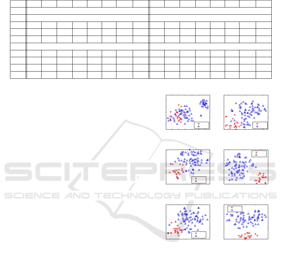
Table 2: Testing performance (%) with/without feature selection (All features/Selected features), as well as with/without

oversampling, on the I, O, and OI features. In case of feature selection, we also consider the omics imaging features (OpI)

obtained by concatenating the I and O features separately selected.

Data Acc Sens Spec Prec F

Gm AUC AGF Acc Sens Spec Prec F

Gm AUC AGF

Testing WITH oversampling Testing WITHOUT oversampling

All features All features

I 67.3 87.0 61.5 40.8 54.7 70.2 74.2 75.2 72.7 82.0 69.9 46.2 57.7 72.2 76.0 75.5

O 92.1 93.0 91.9 81.7 84.9 91.8 92.5 92.5 91.2 70.0 97.4 90.0 75.8 79.7 83.7 79.7

OI 89.8 98.0 87.4 74.3 82.7 92.2 92.7 93.5 93.3 90.0 94.2 86.3 85.9 91.3 92.1 91.7

Selected features Selected features

I 80.5 69.5 83.7 58.2 60.3 70.6 76.6 71.7 81.2 60.4 87.3 58.2 56.3 64.9 73.9 65.5

O 95.1 90.7 96.5 90.8 88.9 92.2 93.6 92.5 94.3 84.9 97.1 90.3 85.4 88.6 91.0 88.7

OI 95.0 91.1 96.1 90.2 88.8 92.4 93.6 92.7 94.6 86.0 97.1 90.5 86.2 89.3 91.5 89.5

OpI 92.8 90.1 93.7 85.3 85.2 90.6 91.9 91.2 92.4 82.0 95.5 86.4 81.4 86.0 88.7 86.3

From Table 2, it can be observed that feature se-

lection almost always leads to a substantial improve-

ment according to any performance measure. Excep-

tions can be observed for Sensitivity in testing with

oversampling (bottom-left of Table 2), which is re-

duced from 87%, 93%, and 98% to 69.5%, 90.7%,

and 91.1% for the I, O, and OI features, respectively.

Consequently, also AGF is reduced, as it weighs more

the correct classiﬁcation of minority samples. How-

ever, these performance reductions are compensated

in terms of augmented values for all the other met-

rics. Instead, in case of results obtained without over-

sampling (right part of Table 2), we can observe more

cases where performance decreases when using fea-

ture selection, especially for the imaging features.

The beneﬁcial role of feature selection is con-

ﬁrmed by the visual analysis based on T-distributed

Stochastic Neighbor Embedding (t-SNE), reported

in Fig. 6. t-SNE is a nonlinear dimensional-

ity reduction technique that allows embedding of

high-dimensional data for visualization in a low-

dimensional space (van der Maaten and Hinton,

2008). It models each high-dimensional sample by

a two- or three-dimensional point in such a way that

similar samples are modeled by nearby points and dis-

similar samples are modeled by distant points with

high probability. It is capable of retaining the local

structure of the high-dimensional data, while also re-

vealing some important global structure, such as the

presence of clusters at several scales. Figs. 6-(a)-(c)

provide visual representations of the glioma data used

for training mapped into the 2D Euclidean space by t-

SNE, considering both all the features (left plots) and

the selected features (right plots). Data are colored

to reﬂect the ground truth classiﬁcation (red squares

for GBM and blue triangles for LGG). In addition

to showing these scatterplots, we also display a met-

ric called neighborhood hit (NH) (Paulovich et al.,

2008). For a given number of neighbors k (in our ex-

-4 -2 0 2 4 6

All features

-10

-8

-6

-4

-2

t-SNE (NH = 0.785185)

GBM

LGG

-5 0 5

Selected features

-5

t-SNE (NH = 0.912963)

GBM

LGG

(a)

-5 0 5

All features

-10

-5

t-SNE (NH = 0.916667)

GBM

LGG

-5 0 5

Selected features

-6

-4

-2

t-SNE (NH = 0.994444)

GBM

LGG

(b)

-6 -4 -2 0 2 4

All features

-10

-5

t-SNE (NH = 0.911111)

GBM

LGG

-4 -2 0 2 4

Selected features

-10

-5

t-SNE (NH = 1.000000)

GBM

LGG

(c)

Figure 6: Role of feature selection: t-SNE of (a) I, (b) O,

and (c) OI data considering all the features (left plots) or

the selected features (right plots) for training data, where

feature selection is performed.

periments, k=6), the NH for a projected point p ∈ R

is deﬁned as the ratio of its k-nearest neighbors (ex-

cept p itself) that belong to the same class as the cor-

responding observation. The NH for a projection is

deﬁned as the average NH over all its points. Intu-

itively, a high NH corresponds to a projection where

the real classes (ground truth) are visually well sep-

arated. Therefore, as suggested in (Rauber et al.,

2018), the NH metric provides a good quantitative

characterization of a t-SNE projection. Fig. 6-(a) re-

ports the t-SNE visual representations for one of the

Glioma Grade Classiﬁcation via Omics Imaging

random partitions of the imaging data. Here, we ob-

serve that the two classes do not appear well sepa-

rated when using all the features (left plots). Instead,

using the subset of selected features (right plots) al-

lows to better group data belonging to the same class

in periphery areas of the 2D plane, even though the

groups are still not spatially separated. The gain in us-

ing feature selection is well reﬂected by the increase

in the NH value. From the visual representations for

the omics data reported in Fig. 6-(b), we observe that

the two classes appear better separated than for the

imaging data, also when using all the features. Using

the subset of selected features leads to data clusters

that are much more spatially separated, also showing

much higher NH values. Similar observations can be

done for the omics imaging data, whose t-SNE visual

representations are reported in Fig. 6-(c), showing

that the subset of selected features leads to correctly

cluster the mapped data in separate plane regions in a

way that is consistent with their classiﬁcation and the

NH values when using only the selected features are

extremely high.

The above analysis based on both performance

metrics and visual representations by t-SNE high-

lights the higher discriminating power of omics imag-

ing data, especially if coupled with feature selection

and oversampling, as compared to any of the types of

data separately.

3.2.1 Comparisons with Other Methods

To complete our analysis and discussion of the pro-

posed framework, we wish to compare our results

with those obtained by different approaches. How-

ever, due to the novelty of our omics imaging ap-

proach, to the best of our knowledge, no other method

exists that has been evaluated on the same dataset

and that can be compared for glioma grade classiﬁ-

cation. Therefore, in Table 3, we summarize the per-

formance of several methods for classifying glioma

grades, bearing in mind that each has been validated

by its authors on a different set of data.

The method in (Law et al., 2003) uses relative

cerebral blood volume (rCBV) measurements derived

from perfusion MRI and metabolite ratios from pro-

ton MR spectroscopy, with a cohort of 160 patients.

Table 3 reports sensitivity and speciﬁcity for discrim-

inating the 120 HGG and 40 LGG samples (computed

by the authors for correct identiﬁcation of HGGs,

i.e., assuming HGG as positive) achieved both using

solely rCBV and combining rCBV with metabolite ra-

tios (m.r.).

The work in (Togao et al., 2016) investigates the

diagnostic performance of intravoxel incoherent mo-

tion imaging for glioma grade classiﬁcation using

Table 3: Performance (%) of methods for glioma grades

classiﬁcation.

Method Acc Sens Spec AUC

Law2003-rCBV 95.0 57.5

Law2003-rCBV+m. r. 93.3 60.0

Togao2016 96.6 81.2 95.0

Zacharaki2009 87.8 84.6 95.5 89.6

Cho2018 88.5 95.1 70.2 90.3

Ertosun2015 96.0 98.0 94.0

Khawaldeh2018 91.3 87.5 95.3

I 80.5 69.5 83.7 76.6

O 95.1 90.7 96.5 93.6

OI 95.0 91.1 96.1 93.6

several parameters, with a cohort of 45 patients. Ta-

ble 3 reports their best sensitivity, speciﬁcity, and

AUC values for discriminating the 29 HGG and 16

LGG samples, obtained based on the volume fraction

within a voxel of water ﬂowing in perfused capillars.

The method in (Zacharaki et al., 2009) is based

on a total of 161 imaging features, including shape,

intensity, and texture features, extracted by different

MRI modalities on a set of 74 brain tumors. Fea-

ture selection is obtained using a SVM-based recur-

sive feature elimination process similar to the one we

adopted, but using a leave-one-out CV. Table 3 reports

the accuracy, sensitivity, speciﬁcity, and AUC values

achieved by weighted SVM to differentiate between

the 22 LGG and 52 HGG samples.

Cho et al. (Cho et al., 2018) quantify gliomas

with a radiomics approach and use the results to dif-

ferentiate between 210 GBM and 75 LGG samples.

They consider data from the MICCAI Brain Tumor

Segmentation 2017 Challenge (Menze et al., 2015),

derived from the TCGA-GBM and TGCA-LGG col-

lections. A set of 468 quantitative radiomics features

(based on shape, histogram, texture, and intensity)

is computed from four MRI modalities, considering

three glioma sub-regions. The minimum redundancy

maximum relevance algorithm is adopted to select

ﬁve features, used to build three different classiﬁer

models. Table 3 reports the average accuracy, sen-

sitivity, speciﬁcity, and AUC values achieved by the

classiﬁers in the testing cohort as deﬁned in the BraTS

challenge.

Two deep learning-based methods have recently

been proposed for classifying glioma grades. In (Er-

tosun and Rubin, 2015), a deep learning-based clas-

siﬁcation pipeline is proposed using digital pathology

images of whole tissue slides obtained by TCGA. Ta-

ble 3 reports the accuracy, sensitivity, and speciﬁcity

values obtained by the authors to differentiate be-

tween the 52 LGG and 48 GBM microbiopsy samples

randomly selected from independent test slides. Deep

BIOIMAGING 2020 - 7th International Conference on Bioimaging

learning-based classiﬁcation for grading of glioma tu-

mors is also considered in (Khawaldeh et al., 2018).

However, the model is trained using single 2D slices

of FLAIR MRI images available in TCIA. The label-

ing available for each patient was extended to label,

for each MRI, a subset of slices showing the lesion.

Table 3 reports the accuracy, sensitivity, and speci-

ﬁcity values computed by the confusion matrix pub-

lished by the authors for a (more difﬁcult) three-class

classiﬁcation problem on 587 samples (213 GBM,

235 LGG, and 139 healthy).

For direct comparison, in Table 3, we also re-

port the best performance results for the proposed ap-

proach using feature selection and oversampling on I,

O, and OI features. Overall, we can conclude that the

proposed approach based on using OI features shows

performance similar to or higher than all the com-

pared methods in terms of all the considered perfor-

mance metrics.

3.3 Analysis of Selected Features

Table 4 reports the most frequently selected features

from I, O, and OI data, respectively. These have been

collected, for each dataset, as those selected in the

training set of each of the 50 iterations of the eval-

uation procedure. The numbers on the left indicate

the number of times (over 50) each feature has been

selected. Among the 704 imaging features (named ac-

cording to the nomenclature provided by the authors

(Bakas et al., 2017b; Bakas et al., 2017c)), only 193

of them have been selected at least once when pro-

cessing imaging data. The most frequently selected

concern volume, histogram, intensity, spatial, and tex-

tural properties of the MRI images. Among the 1375

omics features (named according to the acronyms of

the involved metabolites), only 153 of them have been

selected at least once when processing omics data.

Only 131 of the 2079 omics imaging features have

been selected at least once when processing omics

imaging data. Among them, the most frequently se-

lected imaging features concern volume and spatial

properties, while the most frequently selected omics

features are also those most frequently chosen while

applying feature selection to O alone.

The strategy of integrating omics data into

metabolic models is proper to systems biology ap-

proach, where the integration of multiple informa-

tion coming from different data sources is exploited

to investigate the links among molecular components

of varying nature. Here we used the gene expres-

sion data and the gene-protein-reaction relationships

(GPR) to weight the connections among metabolites

consumed and produced in enzymes-catalyzed reac-

tions. Through this approach, we can get insights

into the metabolism even starting from gene-level

data. Indeed, the extracted features are metabolites

connections, and thus, we can recover useful infor-

mation from single metabolites, whole reactions, be-

longing subsystems, and enzymes, providing a wider

choice of candidate biomarkers. Furthermore, focus-

ing our attention on metabolites, we aim at overcom-

ing the limit imposed by gene expression quantiﬁca-

tion, which requires the extraction of the RNA from

the brain tissue. Indeed, it is possible to measure the

metabolites abundance through LC-MS/MS-based

quantiﬁcation in both cerebrospinal ﬂuid and brain

(Fuertig et al., 2016), through in-vivo proton magnetic

resonance spectroscopy (1H-MRS) (Jansen et al.,

2006). The ﬁrst three mostly recurrent features ob-

tained from omics and omics imaging are exactly the

same, conﬁrming their strong discriminative power.

In particular, the ﬁrst two are selected in almost all

the iterations, and the third one in half of them. All

features highlight an increased nutrient request in

more aggressive cancers, made of cells that prolifer-

ate and invade more rapidly. Indeed, the ﬁrst metabo-

lite couple (m00247c m00569c), 1,3-bisphospho-D-

glycerate → 2,3-bisphospho-D-glycerate, is part of

the Glycolysis/Gluconeogenesis subsystem, and the

associated reaction is catalyzed by PGAM1. The lat-

ter is the brain isoform of the phosphoglyceric acid

mutase, a well-known enzyme in cancer research,

since it is involved in the so-called Warburg effect,

the aerobic glycolisis that provides a selective ad-

vantage to cancer cells for growing and proliferat-

ing. Its abundance is highly correlated to aggres-

siveness and poor prognosis of tumors (Sun et al.,

2018). The second omics and omics imaging feature

(m02579c m02579s) is the transport of ammonium

ions NH4+ from cytoplasm to extracellular compart-

ment. Several studies have associated ammonium

ions to growth, death, and regulation of apoptotic pro-

cesses, depending on cell types. It is generally rec-

ognized as a waste product of glutaminolysis, a fun-

damental energy source for proliferating cells, and is

deleterious to cells; that is the reason for ﬁnding the

transport toward the outside of cells. Surely NH4+

abundance and transport are correlated to the rate of

energy production (Abusneina and Gauthier, 2016).

The third metabolites link (m01972l m01430l) in-

volves the following reaction: glucosylceramide pool

+ H2O → ceramide pool + glucose. It is part of the

glycosphingolipid metabolism in lysosomes, which

are lipids particularly abundant in the nervous system,

involved in many biological processes. The impair-

ment of their production or catabolism leads to differ-

ent lysosome storage diseases, which are a hallmark

Glioma Grade Classiﬁcation via Omics Imaging

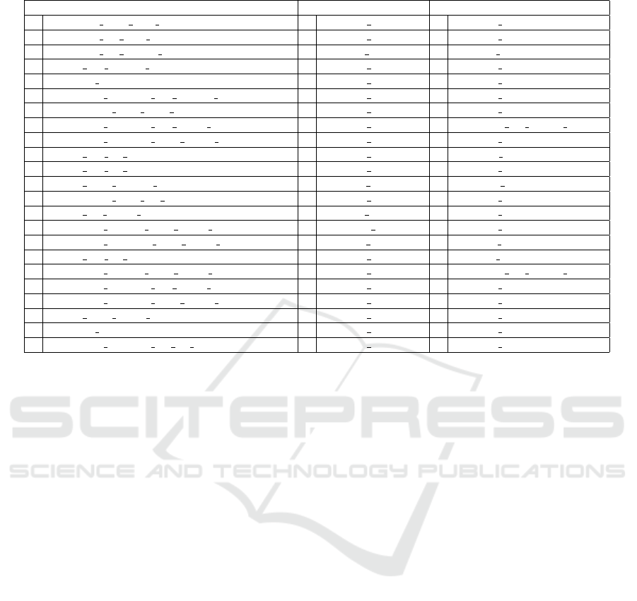
Table 4: Most frequently selected imaging, omics, and omics imaging features, with their frequency.

Imaging Omics Omics&Imaging

36 VOLUME NET over TC 49 m00247c m00569c 47 m00247c m00569c

32 VOLUME ET over TC 47 m02579c m02579s 43 m02579c m02579s

30 VOLUME ET OVER WT 24 m01972l m01430l 28 m01972l m01430l

26 HISTO ED FLAIR Bin10 23 m01990c m01992c 24 m01688c m01680c

25 SPATIAL Temporal 21 m02133c m02471c 23 m02344c m02344s

25 TEXTURE GLSZM ED FLAIR SZHGE 20 m02344c m02344s 19 m01990c m01992c

23 INTENSITY STD NET T1Gd 19 m01688c m01680c 18 m02133c m02471c

21 TEXTURE GLSZM ED T1Gd LGZE 18 m02845c m02806c 12 VOLUME ET OVER WT

21 TEXTURE GLSZM NET T1Gd SZHGE 15 m01307c m02335c 11 m00809c m00968c

18 HISTO ED T1 Bin3 13 m01972c m01430c 11 m01868g m01869g

16 HISTO ED T1 Bin2 11 m01939c m00247c 11 m02658c m02812c

16 HISTO NET FLAIR Bin10 10 m01913s m01910s 10 SPATIAL Insula

15 INTENSITY STD ET T1Gd 9 m01307c m02818c 10 m01115c m02471c

14 HISTO ET T1Gd Bin7 9 m02008l m01910l 10 m01939c m00247c

14 TEXTURE GLCM NET T1Gd AutoCorrelation 8 m00826m m02189m 10 m01965c m01965g

14 TEXTURE GLRLM NET T1Gd SRLGE 8 m01821s m01822s 9 m01913s m01910s

13 HISTO ED T1 Bin6 8 m01965c m01965g 9 m02008l m01910l

13 TEXTURE GLCM NET T1Gd SumAverage 8 m02658c m02812c 7 VOLUME ET OVER BRAIN

12 TEXTURE GLSZM ED T1Gd SZLGE 7 m00351c m00349c 7 m00554c m00555c

10 TEXTURE GLSZM NET T1Gd SZE 7 m00809c m00968c 7 m01307c m02335c

9 HISTO NET T1Gd Bin10 7 m01968c m01968r 7 m01673c m01755c

9 SPATIAL Insula 6 m00554c m00555c 7 m01690c m01939c

9 TEXTURE GLSZM ET T2 SZHGE 6 m01690c m01939c 7 m02845c m02806c

of neuronopathic forms of the disease (Boomkamp

and Butters, 2008; Russo et al., 2018).

4 CONCLUSIONS

The availability of data from both omics and imaging

experiments for each patient provides deeper insight

into the classiﬁcation of disease states, as in the case

of brain tumors. In this work, we analyze in detail

the problem of integrating publicly available data to

discriminate between brain tumor subtypes. Imaging

features come from analyses available in the TCIA

archive, while, in the case of transcriptomic data, fea-

tures are extracted in terms of metabolic information

through the integration of gene expression values into

a genome-wide metabolic model of the brain tissue.

This approach allows us to get a broader range of in-

formation, going from the enzymes to the metabo-

lites and the associated reactions. Focusing on the

metabolic alterations is a widespread strategy in can-

cer research, both because the transformed cells adopt

an energy/metabolic reprogramming (Jeon and Hay,

2018) and because the metabolites and the enzymes

represent good targets for diagnostic and therapeu-

tic challenges (Luengo et al., 2017). The adopted

framework takes into account several strategies that

can lead to better and fairer results, including feature

selection and data balancing, and their correct incor-

poration in the entire procedure. We show that the

integration of omics and imaging data, also thanks to

these precautions, can provide more accurate results

than their separate use, even using a small number

of signiﬁcant features from both the types of exper-

iments.

Future research will be devoted to both new meth-

ods and data. Indeed, our implementation choices

have been guided by the established literature, rather

than by their speciﬁc suitability for the problem at

hand. It will be interesting to further investigate

whether the adoption of different classiﬁer models,

data balancing strategies or feature selection algo-

rithms speciﬁcally devised for integrating multimodal

data, may lead to even better results for this or sim-

ilar applications. Moreover, we will try to integrate

larger volumes of data coming from different experi-

ments and to generalize our ﬁndings to more massive

datasets of various diseases. This means, on the one

hand, producing imaging features with standard and

FAIR procedures, like those adopted in this study. On

the other hand, this leads our attention to other types

of omics data (e.g., those coming from the blood)

that could help reducing invasive interventions. This

would facilitate and enhance the role of omics imag-

ing studies as a support to the medical doctors.

BIOIMAGING 2020 - 7th International Conference on Bioimaging

ACKNOWLEDGEMENTS

The work was carried out also within the activities

of M.R. Guarracino and L. Maddalena as members

of the INdAM Research group GNCS. M. Manzo ac-

knowledges the guidance and supervision of Prof. Al-

fredo Petrosino during the years spent working to-

gether. The authors would like to thank G. Trerotola

for the technical support.

REFERENCES

Abusneina, A. and Gauthier, E. R. (2016). Ammonium ions

improve the survival of glutamine-starved hybridoma

cells. Cell & bioscience, 6(1):23.

Acharya, U. R., Hagiwara, Y., Sudarshan, V. K., et al.

(2018). Towards precision medicine: from quantita-

tive imaging to radiomics. J. Zhejiang Univ. Sci. B,

19(1):6–24.

Agren, R., Bordel, S., Mardinoglu, A., et al. (2012). Recon-

struction of genome-scale active metabolic networks

for 69 human cell types and 16 cancer types using

INIT. PLoS computational biology, 8(5):e1002518.

Antonelli, L., Guarracino, M. R., Maddalena, L., et al.

(2019). Integrating imaging and omics data: A review.

Biomed Signal Process Control, 52:264–280.

Bakas, S., Akbari, H., Sotiras, A., et al. (2017a). Advancing

The Cancer Genome Atlas glioma MRI collections

with expert segmentation labels and radiomic features.

Scientiﬁc data, 4.

Bakas, S., Akbari, H., Sotiras, A., et al. (2017b). Seg-

mentation labels and radiomic features for the pre-

operative scans of the TCGA-GBM collection. The

Cancer Imaging Archive.

Bakas, S., Akbari, H., Sotiras, A., et al. (2017c). Seg-

mentation labels and radiomic features for the pre-

operative scans of the TCGA-LGG collection. The

Cancer Imaging Archive.

Beig, N. et al. (2017). Radiogenomic analysis of hypoxia

pathway reveals computerized MRI descriptors pre-

dictive of overall survival in glioblastoma. In Proc.

SPIE, volume 10134, pages 101341U–101341U–10.

Boomkamp, S. D. and Butters, T. D. (2008). Glycosphin-

golipid disorders of the brain. In Lipids in Health and

Disease, pages 441–467. Springer.

Chawla, N. V., Bowyer, K. W., Hall, L. O., et al. (2002).

Smote: Synthetic minority over-sampling technique.

J. Artif. Int. Res., 16(1):321–357.

Cho, H.-h., Lee, S.-h., Kim, J., et al. (2018). Classiﬁcation

of the glioma grading using radiomics analysis. PeerJ,

Clark, K. et al. (2013). The Cancer Imaging Archive

(TCIA): Maintaining and operating a public infor-

mation repository.

Journal of Digital Imaging

26(6):1045–1057.

Diehn, M. et al. (2008). Identiﬁcation of noninvasive imag-

ing surrogates for brain tumor gene-expression mod-

ules. Proc. of the National Academy of Sciences of the

United States of America, 105(13):5213–5218.

Ertosun, M. G. and Rubin, D. L. (2015). Automated grad-

ing of gliomas using deep learning in digital pathol-

ogy images: A modular approach with ensemble of

convolutional neural networks. In AMIA 2015 Annual

Symposium Proc., pages 1899–1908.

Fuertig, R., Ceci, A., Camus, S. M., Bezard, E., Luippold,

A. H., and Hengerer, B. (2016). LC–MS/MS-based

quantiﬁcation of kynurenine metabolites, tryptophan,

monoamines and neopterin in plasma, cerebrospinal

ﬂuid and brain. Bioanalysis, 8(18):1903–1917.

Gevaert, O., Mitchell, L., Achrol, A., et al. (2014).

Glioblastoma multiforme: exploratory radiogenomic

analysis by using quantitative image features. Radiol-

ogy, 273(1):168–74.

Gillies, R. J., Kinahan, P. E., and Hricak, H. (2016). Ra-

diomics: Images are more than pictures, they are data.

Radiology, 278(2):563–577. PMID: 26579733.

Granata, I., Guarracino, M. R., Kalyagin, V. A., et al.

(2018). Supervised classiﬁcation of metabolic net-

works. In IEEE Int. Conf. on Bioinformatics and

Biomedicine (BIBM), Madrid, Spain, December 3-6,

2018, pages 2688–2693.

Granata, I., Guarracino, M. R., Kalyagin, V. A., et al.

(2019). Model simpliﬁcation for supervised classiﬁ-

cation of metabolic networks. Annals of Mathematics

and Artiﬁcial Intelligence.

Guyon, I., Weston, J., Barnhill, S., et al. (2002). Gene se-

lection for cancer classiﬁcation using support vector

machines. Machine Learning, 46(1):389–422.

Haibo He, Yang Bai, Garcia, E. A., et al. (2008). ADASYN:

Adaptive synthetic sampling approach for imbalanced

learning. In 2008 IEEE Int. Joint Conf. on Neural Net-

works (IEEE World Congress on Computational Intel-

ligence), pages 1322–1328.

Hariri, A. R. and Weinberger, D. R. (2003). Imaging ge-

nomics. British Medical Bulletin, 65(1):259–270.

He, H. and Garcia, E. A. (2009). Learning from imbalanced

data. IEEE T Knowl Data En, 21(9):1263–1284.

Jaffe, C. C. (2012). Imaging and genomics: Is there a syn-

ergy? Radiology, 264(2):329–331.

Jain, R., Poisson, L., Narang, J., Scarpace, L., et al. (2012).

Correlation of perfusion parameters with genes related

to angiogenesis regulation in glioblastoma: a feasibil-

ity study. AJNR Am J Neuroradiol., 33(7):1343–8.

Jansen, J. F., Backes, W. H., Nicolay, K., and Kooi, M. E.

(2006). 1h MR spectroscopy of the brain: absolute

quantiﬁcation of metabolites. Radiology, 240(2):318–

332.

Jeon, S.-M. and Hay, N. (2018). Expanding the concepts of

cancer metabolism.

Khawaldeh, S., Pervaiz, U., Raﬁq, A., et al. (2018). Non-

invasive grading of glioma tumor using magnetic res-

onance imaging with convolutional neural networks.

Applied Sciences, 8(1).

Kumar, V. et al. (2012). Radiomics: the process

and the challenges. Magnetic Resonance Imaging,

30(9):1234–1248. Quantitative Imaging in Cancer.

Glioma Grade Classiﬁcation via Omics Imaging

Lambin, P., Rios-Velazquez, E., Leijenaar, R., et al. (2012).

Radiomics: Extracting more information from medi-

cal images using advanced feature analysis. European

Journal of Cancer, 48(4):441–446.

Law, M., Yang, S., and Wang, H. a. (2003). Glioma grading:

Sensitivity, speciﬁcity, and predictive values of perfu-

sion MR imaging and proton MR spectroscopic imag-

ing compared with conventional MR imaging. Amer-

ican Journal of Neuroradiology, 24(10):1989–1998.

Lee, G., Lee, H. Y., Ko, E. S., et al. (2017). Radiomics

and imaging genomics in precision medicine. Precis

Future Med, 1(1):10–31.

Louis, D. N., Perry, A., Reifenberger, G., Von Deimling,

A., Figarella-Branger, D., Cavenee, W. K., Ohgaki,

H., Wiestler, O. D., Kleihues, P., and Ellison, D. W.

(2016). The 2016 World Health Organization clas-

siﬁcation of tumors of the central nervous system: a

summary. Acta neuropathologica, 131(6):803–820.

Luengo, A., Gui, D. Y., and Vander Heiden, M. G. (2017).

Targeting metabolism for cancer therapy. Cell chemi-

cal biology, 24(9):1161–1180.

Manzo, M. (2019). Kgearsrg: Kernel graph embedding on

attributed relational sift-based regions graph. Machine

Learning and Knowledge Extraction, 1(3):962–973.

Maratea, A., Petrosino, A., and Manzo, M. (2014). Ad-

justed f-measure and kernel scaling for imbalanced

data learning. Information Sciences, 257:331–341.

Menze, B. H., Jakab, A., Bauer, S., et al. (2015). The mul-

timodal brain tumor image segmentation benchmark

(brats). IEEE Trans Med Imaging, 34(10):1993–2024.

Paulovich, F. V., Nonato, L. G., Minghim, R., et al. (2008).

Least square projection: A fast high-precision mul-

tidimensional projection technique and its application

to document mapping. IEEE Trans Vis Comput Graph,

14(3):564–575.

Peeken, J. C., Bernhofer, M., Wiestler, B., et al. (2018).

Radiomics in radiooncology - challenging the medical

physicist. Physica Medica, 48:27–36.

Ranjbar, S. and Mitchell, J. R. (2017). Chapter 8 - an intro-

duction to radiomics: An evolving cornerstone of pre-

cision medicine. In Depeursinge, A., Al-Kadi, O. S.,

and Mitchell, J., editors, Biomedical Texture Analysis,

pages 223 – 245. Academic Press.

Rauber, P. E., Falcao, A. X., and Telea, A. C. (2018). Pro-

jections as visual aids for classiﬁcation system design.

Information Visualization, 17(4):282–305.

Russo, D., Della Ragione, F., Rizzo, R., Sugiyama, E.,

Scalabr

ı, F., Hori, K., Capasso, S., Sticco, L., Fior-

iniello, S., De Gregorio, R., et al. (2018). Glycosph-

ingolipid metabolic reprogramming drives neural dif-

ferentiation. The EMBO journal, 37(7):e97674.

Sala, E. et al. (2017). Unravelling tumour heterogene-

ity using next-generation imaging: Radiomics, ra-

diogenomics, and habitat imaging. Clin. Radiol.,

72(1):3–10.

Santos, M. S., Soares, J. P., Abreu, P. H., et al. (2018).

Cross-validation for imbalanced datasets: Avoiding

overoptimistic and overﬁtting approaches [research

frontier]. IEEE Comp. Int. Mag., 13(4):59–76.

Smedley, N. F. and Hsu, W. (2018). Using deep neural net-

works for radiogenomic analysis. In 2018 IEEE 15th

Int. Symposium on Biomedical Imaging (ISBI 2018),

pages 1529–1533.

Soeda, A., Hara, A., Kunisada, T., Yoshimura, S.-i., Iwama,

T., and Park, D. M. (2015). The evidence of glioblas-

toma heterogeneity. Scientiﬁc reports, 5:7979.

Sun, Q., Li, S., Wang, Y., Peng, H., Zhang, X., Zheng, Y.,

Li, C., Li, L., Chen, R., Chen, X., et al. (2018). Phos-

phoglyceric acid mutase-1 contributes to oncogenic

mTOR-mediated tumor growth and confers non-small

cell lung cancer patients with poor prognosis. Cell

Death & Differentiation, 25(6):1160.

Togao, O., Hiwatashi, A., Yamashita, K., et al. (2016).

Differentiation of high-grade and low-grade diffuse

gliomas by intravoxel incoherent motion MR imaging.

Neuro-Oncology, 18(1):132–141.

van der Maaten, L. and Hinton, G. (2008). Visualizing data

using t-SNE. Journal of Machine Learning Research,

9:2579–2605.

Vapnik, V. (1995). The Nature of Statistical Learning The-

ory. Springer-Verlag.

Wang, L., Wang, Y., and Chang, Q. (2016). Feature se-

lection methods for big data bioinformatics: A survey

from the search perspective. Methods, 111:21–31. Big

Data Bioinformatics.

Wu, X., Kumar, V., Ross Quinlan, J., et al. (2007). Top 10

algorithms in data mining. Knowl. Inf. Syst., 14(1):1–

37.

Zacharaki, E. I., Wang, S., Chawla, S., et al. (2009). Classi-

ﬁcation of brain tumor type and grade using MRI tex-

ture and shape in a machine learning scheme. Magn

Reson Med, 62:a609–1618.

Zinn, P., Majadan, B., et al. (2011). Radiogenomic map-

ping of edema/cellular invasion MRI-phenotypes in

glioblastoma multiforme. PLoS ONE, 6(10).

BIOIMAGING 2020 - 7th International Conference on Bioimaging