A New Diversity Maintenance Strategy based on the Double Granularity

Grid for Multiobjective Optimization

Junzhong Ji, Yannan Weng and Cuicui Yang

College of Computer, Beijing University of Technology, Beijing Municipal Key Laboratory of Multimedia and Intelligent

Software, Beijing Artiﬁcial Intelligence Institute, Pingleyuan 100, Chaoyang District, Beijing, China

Keywords:

Multiobjective Optimization, Diversity Maintenance, Double Granularity Grid.

Abstract:

The diversity maintenance of nondominated solutions is crucial for solving multiobjective optimization prob-

lems. The grid strategy is a very effective way to maintain the diversity of nodominated solutions, but the

existing grid strategies all adopt single-layer grid structure, which has weak ability for judging the distribution

of nodominated solutions in the hyperboxes with the same crowding degree. To further explore the ability of

the grid strategy for maintaining the diversity of nondominated solutions, this paper presents a new diversity

maintenance strategy based on the double granularity grid. The double granularity grid strategy ﬁrstly parti-

tions the hyperboxes with the same largest crowding degree into ﬁne granularity hyperboxes. Then, it selects

nondominated individual solutions according to the solution distribution in both coarse and ﬁne granularity

hyperboxes, which can avoids randomness for selecting individual solutions in the single grid structure. To

validate the performance of the double granularity grid strategy, we ﬁrst integrated it with two famous algo-

rithms, then tested the two integration algorithms by comparing them with the original algorithms and four

other state-of-the-art algorithms.The experimental results validate the powerful advantages of the proposed

double granularity grid strategy.

1 INTRODUCTION

Multiobjective optimization problems (MOPs) con-

sist of multiple conﬂicting objectives that need to

be optimized simultaneously, and widely exist in so-

cial life and engineering applications (Deb, 2001;

Deb, 2014). Generally, there is no single solu-

tion for MOPs, but rather a set of alternative so-

lutions, called Pareto optimal solutions or nondom-

inated solutions. Population evolution-based algo-

rithms including evolutionary and swarm intelligence

algorithms, which are considered to be very suit-

able for solving MOPs due to their property of

achieving an approximation of the Pareto in a single

run (Aimin Zhou and Zhang, 2011; Margarita and

Coello, 2006), and such algorithms are called evo-

lutionary multiobjective optimization (EMO) algo-

rithms. Over the past few decades, some well-known

EMO algorithms have been proposed, such as NSGA-

II (K. Deb and Meyarivan, 2000), IBEA (Eckart

and K

unzli, 2004), PESA-II (Corne D W, 2001),

MOEA/D (Zhang and Li, 2007), MOPSO (Coello

et al., 2004), NSLS (Bili Chen and Zhang, 2015) and

so on. Usually, these algorithms pursue two goals:

minimizing the distance between the obtained Pareto

front and true the Pareto front (ie., convergence) and

maximizing the distribution of the obtained Pareto op-

timal solutions (ie., diversity) (Ge et al., 2019). That

is, most EMO algorithms need to balance both con-

vergence and diversity in order to get a set of uni-

formly distributed optimal solutions. Clearly, it is

very important to keep the diversity of nondominated

solutions found in the optimization. Up to now, re-

searchers have proposed different diversity mainte-

nance strategies, including niche, clustering, kth near-

est distance and grid (Li et al., 2014).

In the existing diversity maintenance strategies,

the grid strategy has an inherent property of reﬂect-

ing the diversity of individuals in a population (Yang

et al., 2013; X. Cai and Zhang, 2017). Corne and

Knowles developed PAES algorithm (Pareto Archive

Evolution Strategy) (JD and DW, 2000), which is

the ﬁrst algorithm to introduce the grid strategy to

maintain the diversity of the nondominated solutions.

Afterwards, they proposed other two different algo-

rithms, PESA (The Pareto Envelope-based selection

algorithm) (Corne et al., 2000) and PESA-II (Corne

D W, 2001), based on the grid strategy. PESA adopts

individual selection based on the grid strategy, and

PESA-II uses region selection. Coello et al. pre-

Ji, J., Weng, Y. and Yang, C.

A New Diversity Maintenance Strategy based on the Double Granularity Grid for Multiobjective Optimization.

DOI: 10.5220/0009167500880095

In Proceedings of the 9th International Conference on Pattern Recognition Applications and Methods (ICPRAM 2020), pages 88-95

ISBN: 978-989-758-397-1; ISSN: 2184-4313

sented MOPSO algorithm (Handling Multiple Ob-

jectives With Particle Swarm Optimization) (Coello

et al., 2004), which adopted the adaptive grid strategy

to preserve the diversity of nondominated solutions.

These existing grid-based algorithms have proved the

validity of the grid strategy in maintaining the diver-

sity of nondominated solutions. However, these algo-

rithms only use single-layer grid structure, and ran-

domly select a hyperbox or an individual when mul-

tiple hyperboxes contain the same amount of individ-

uals, which may undermine the diversity of the non-

dominated solutions in the crowded area.

To further explore the ability of the grid strat-

egy for maintaining the diversity of nondominated so-

lutions, this paper presents a novel diversity main-

tenance strategy based on the double granularity

grid(DGG) strategy. The DGG strategy partitions

the hyperboxes with the same largest crowding de-

gree into ﬁne granularity hyperboxes to more pre-

cisely locate the position of the nondominated solu-

tions, which can avoid randomness for selecting hy-

perboxes and individual solutions in the single grid

structure.

To verify the effectiveness of DGG strategy, we

ﬁrst integrated it into two algorithms based on the

single-layer grid structure to generate two new inte-

gration algorithms. Then tested the two new inte-

grated algorithms by comparing them with the orig-

inal algorithm and four other EMO algorithms.

The rest of this paper is organized as follows.

Section 2 brieﬂy introduces basic concepts involving

MOPs. Section 3 is devoted to describing the details

of the proposed method. Next, Section 4 presents the

experimental design and results. Section 5 concludes

this paper and outlines future research directions.

2 BASIC CONCEPTS

Without loss of generality, a MOP may be stated as

a minimization problem and deﬁned as follows (Deb,

2001):











min y = F(x) = ( f

(x), f

(x),· ·· , f

(x))

s.t. g

(x) ≤ 0,i = 1,2, ··· , p

(x) = 0, j = 1,2, ·· · ,q

≤ x

(1)

where x = (x

,·· · ,x

) ∈ X ⊂ R

is a n-dimensional

decision vector, X represents a n-dimensional deci-

sion space, x

and x

are the upper and lower bound-

ary values of x

, respectively. y = (y

,·· · ,x

) ∈

Y ⊂ R

is a m-dimensional objective vector, Y rep-

resents a m-dimensional objective space. F(x) is a

mapping function from n-dimensional decision space

to m-dimensional objective space. g

(x) ≤ 0 (i =

1,2,· ·· , p) and h

(x) = 0 ( j = 1,2,·· · ,q) deﬁnes p

inequalities and q equalities, respectively.

In the following, we will list four deﬁnitions in-

volving MOPs.

Deﬁnition 1 (Pareto Dominant). x

, x

are two

feasible solutions, x

is Pareto dominant compared

with x

if and only if:

∀i = 1,2,· ·· , m, f

) ≤ f

) ∧

∃ j = 1, 2,· ·· ,m, f

) < f

)

. (2)

We call this relationship x

 x

, x

dominate x

, or

is dominated by x

Deﬁnition 2 (Pareto Optimal Solution). Ω is the

feasible solution set, x

∗

∈ Ω, x

∗

is a Pareto optimal

solution if and only if:

¬∃x ∈ Ω : x  x

∗

. (3)

Deﬁnition 3 (Pareto Optimal Set). The Pareto

optimal set includes all the Pareto optimal solutions

and is given as follows:

∗

= {x

∗

|¬∃x ∈ Ω : x  x

∗

}. (4)

Deﬁnition 4 (Pareto Front). The Pareto front

(noted as PF) includes all the objective vectors cor-

responding to X

∗

and is given as follows:

PF ={F(x

∗

)= ( f

∗

), f

∗

),· ·· , f

∗

))

∗

∈X

∗

(5)

For better distinction, we present the true PF and the

PF obtained by an algorithm as PF

true

and PF

approx

respectively.

3 DOUBLE GRANULARITY GRID

(DGG) STRATEGY

Usually, the EMO algorithms set in two populations:

an internal population and an external population

(also called archive set (EA)). The internal population

executes optimization mechanisms, and the external

population preserves the nondominated solutions ob-

tained in the optimization process. When the size of

EA exceeds the speciﬁed quantity, the DGG strategy

is used to remove redundant solutions and maintain

the diversity of nondominated solutions. As shown

in the Strategy 1, implementation of this strategy in-

cludes the following two steps.

Step 1) Coarse Granularity Grid Partition.

The objective space region is divided into coarse

granularity that EA occupies into hyperboxes, and

div1 represents the number of ﬁrst partition for each

dimensional objective space. At the same time, some

relevante information, including the lower and upper

boundaries of the grid, the width and grid coordinate

A New Diversity Maintenance Strategy based on the Double Granularity Grid for Multiobjective Optimization

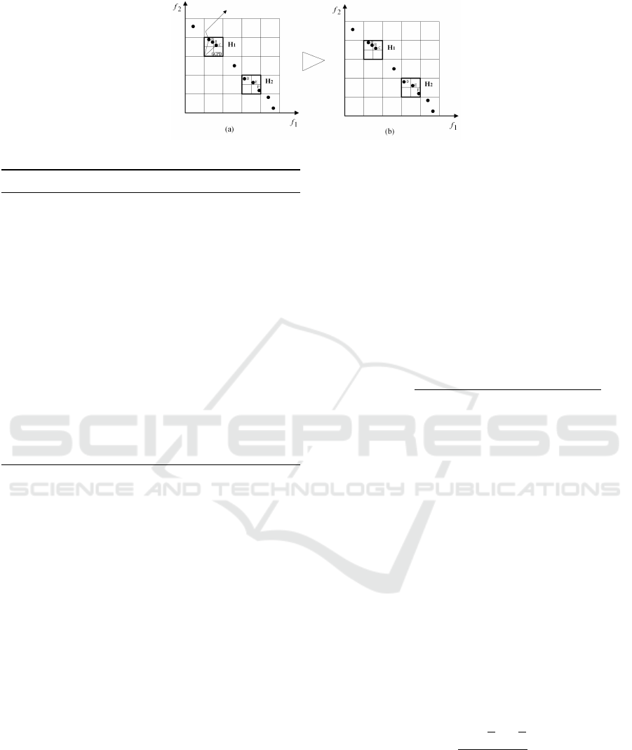
Figure 1: Schematic diagram of the double granularity grid strategy.

Strategy 1: Double Granularity Grid Strategy.

1 while EA exceeding speciﬁed quantity

2 Make a coarse granularity partition on the objective

space region that EA occupy.

3 i) If only one coarse hyperbox has the highest crowding

degree (denoted by δ)

4 • Compute the GCPD of each individual in this

coarse hyperbox as Eq.(10);

5 • Remove the individual with the largest value of

GCPD.

6 ii) If more than one coarse hyperbox have the same δ

7 • Make a ﬁne granularity partition on the coarse

hyperboxes;

8 • Calculate the E of these coarse hyperboxes based

on the δ of ﬁne hyperboxes as Eq.(11);

9 • Select the coarse hyperbox with the smallest

value of E;

10 • Remove the individual with the largest value of

GCPD in the selected coarse hyperbox.

11 end while

of each dimensional objective for each coarse granu-

larity hyperbox, is provided. Each individual solution

in EA has an exact position in a coarse granularity

hyperbox. Each coarse granularity hyperbox has a

crowding degree attribute denoted by δ, which rep-

resents the total number of individual solutions con-

tained in this coarse granularity hyperbox. In ad-

dition, each coarse granularity hyperbox has a m-

dimensional grid coordinate, and its kth grid coordi-

nate is deﬁned as follows.

For the kth objective, the lower and upper bound-

aries of the grid are determined according to the fol-

lowing formula:

=min

(EA)−(max

(EA)−min

(EA))/(2 ∗ div1) (6)

=max

(EA)+(max

(EA)−min

(EA))/(2∗div1) (7)

where max

(EA) and min

(EA) stand for the minimal

and maximal values in the kth objective, respectively.

The coarse granularity hyperbox width in the kth

objective can be formed as:

= (ub

− lb

)/div1 (8)

The grid coordinates of an individual on the kth

objective is deﬁned as:

(x) = f loor(( f

(x) − lb

)/d

) (9)

where f

(x) is the actual kth objective value.

Step 2) Fine Granularity Grid Partition. When

the EA exceeds the speciﬁed size, the individual in

coarse granularity hyperbox with maximum crowd-

ing degree is continuously reduced one by one until

the capacity of EA reaches the speciﬁed number. If

only one coarse granularity hyperbox has the maxi-

mum crowding degree, calculate the grid coordinate

point distance (GCPD) for each individual in the hy-

perbox, and then select the individual with the highest

GCPD value to delete. Here GCPD is a useful criteria

to discriminate individuals in the same hyberbox, and

is deﬁned as (Yang et al., 2013):

GCPD(x)=

∑

k=1

(( f

(x)−(lb

(x) ∗ d

))/d

)

(10)

where m is the number of objectives.

There is another situation where multiple coarse

granularity hyperboxes have the same maximum

crowding degree. In this case, ﬁrst divide those coarse

granularity hyperboxes further with partition number

div2 and calculate the crowding degree of each ﬁne

granularity hyperbox. Then, according to the crowd-

ing degree of ﬁne granularity hyperboxes, calculate

the evenness index of the corresponding coarse gran-

ularity hyperbox and choose the coarse granularity

hyperbox with the smallest evenness index. At last,

compute the GCPD value of all the individual so-

lutions in the selected coarse granularity hyperbox

and remove the one with largest value of GDPD. The

evenness index is diffusely used to measure the even-

ness of individual solutions distribution in a popula-

tion and is deﬁned as (E. Elejalde and Bollen, 2018):

E =

−

∑

i=1

∗ ln

lnC

(11)

where C is the number of ﬁne granularity hyperboxes

in the coarse granularity hyperbox, and C = (div2)

N is the crowding degree of the coarse granularity hy-

perbox, n

is the crowding degree of the ﬁne granular-

ity hyperbox i.

From the above can be obtained, compared with

the single-layer grid structure, the proposed DGG

ICPRAM 2020 - 9th International Conference on Pattern Recognition Applications and Methods

Table 1: Comparison results of PESA-II and PESA-II+DGG on the UF suit.

Problems

IGD HV

PESA-II PESA-II+DGG PESA-II PESA-II+DGG

UF1

1.6746E−1(5.26E−2) 1.5827E−1(4.77E−2) 5.3944E−1(4.43E−2) 5.5198E−1(4.77E−2)

UF2

8.1915E−2(2.28E−2) 7.5380E−2(2.44E−2) 6.3582E−1(1.35E−2) 6.3947E−1(1.69E−2)

UF3

3.0906E−1(3.65E−2) 3.0581E−1(3.72E−2) 3.9149E−1(4.26E−2) 3.9866E−1(3.00E−2)

UF4

5.4234E−2(2.42E−3) 5.3642E−2(1.29E−3) 3.6967E−1(3.89E−3) 3.6973E−1(2.41E−3)

UF5

9.3133E−1(2.42E−1) 8.6005E−1(2.01E−1) 4.1482E−3(1.25E−2) 4.8915E−3(1.20E−2)

UF6

3.4004E−1(1.30E−1) 3.2328E−1(1.26E−1) 2.3587E−1(6.43E−2) 2.4043E−1(6.96E−2)

UF7

3.1960E−1(1.52E−1) 2.9626E−1(1.93E−1) 3.2372E−1(9.32E−2) 3.4040E−1(1.19E−1)

Table 2: Comparison results of PESA-II and PESA-II+DGG on the DTLZ suit.

Problems

IGD HV

PESA-II PESA-II+DGG PESA-II PESA-II+DGG

DTLZ1

2.8645E−2(5.00E−2) 1.9636E−2(1.59E−2) 8.0912E−1(1.17E−1) 8.2774E−1(7.97E−3)

DTLZ2

5.7137E−2(7.95E−3) 5.6004E−2(6.27E−3) 5.4325E−1(7.99E−3) 5.4030E−1(7.32E−3)

DTLZ3

1.4474E+0(1.41E+0) 1.3363E+0(1.20E+0) 1.5604E−1(2.28E−1) 1.5676E−1(2.40E−1)

DTLZ4

5.4250E−2(3.53E−3) 5.2816E−2(3.13E−3) 5.4765E−1(8.46E−3) 5.4795E−1(6.81E−3)

DTLZ5

4.4671E−3(3.92E−4) 4.3857E−3(2.79E−4) 1.9874E−1(2.06E−3) 1.9916E−1(9.33E−4)

DTLZ6

5.0470E−3(3.08E−4) 4.9680E−3(2.52E−4) 1.9827E−1(2.05E−3) 1.9831E−1(1.98E−3)

DTLZ7

5.4475E−2(5.61E−2) 4.4917E−2(1.74E−3) 2.7794E−1(7.08E−3) 2.7853E−1(2.78E−3)

strategy has two differences. On the one hand, when

there are multiple coarse granularity hyperboxes with

largest crowding degree, they are further divided into

ﬁne granularity hyperboxes. On the other hand,

GCPD is used as the basis for individual selection.

Therefore, the DGG strategy enhances the resolution

of the hyperbox, avoids the randomness of the hyper-

box and solution selection, and enables the distribu-

tion of nondominated solutions more uniform.

For clarity, Fig.1 shows a simple two-dimensional

example. Fig.1 (a) gives an EA that holds all non-

dominated solutions, the number of solutions which

exceed the maximum capacity of the EA is 1. Thus,

the DGG strategy is used to eliminate one redundant

solution. Firstly, divide the objective space of the EA

to get coarse granularity hyperboxes with the partition

number of 5, and ﬁnd the coarse granularity hyperbox

with the largest crowding degree. As shown in Fig.1

(a), H

and H

are the two coarse granularity hyper-

boxes with biggest crowding degree, which consists

of three individuals. Secondly, a ﬁne granularity par-

tition in H

and H

for ﬁne granularity hyperbox, the

number of partitions is 2 and calculate the evenness

of H

and H

, select the H

with smaller evenness

according to Eq.(10). Finally, compute the GCDP of

individual A, B and C in the coarse granularity hyper-

box H

according to Eq.(11), choose the individual A

with the largest value and remove it from the EA, and

obtain the ﬁnal nondominated solution set as shown

in Fig.1(b).

4 EXPERIMENTS

In this section, extensive experiments have veri-

ﬁed the performance of the proposed DGG strat-

egy. The experimental platform is a PC with In-

tel(R) Core(TM) i5-4590 CPU 3.30GHz, 8GB RAM,

and Windows 10, and DGG is implemented using the

Matlab language.

4.1 Experimental Setting

Two well-deﬁned test suites, the UF (Huband et al.,

2005) and DTLZ (K. Deb and Zitzler, 2005), are se-

lected in this paper. UF1-UF7 are bi-objective test

problems, and DTLZ1-DTLZ7 are tri-objective test

problems to further examine the performance of the

DGG strategy in handling MOPs with more than two

objectives. We chose two evaluation metrics: the

inverted generational distance(IGD) (Bosman and

Thierens, 2003) and hypervolume (HV) (Z. Eckart

and Lothar, 2008), which can check convergence and

diversity simultaneously.

Let S

∗

be a set of uniformly distributed solutions

along PF

true

and S be the set of obtained solutions

along PF

approx

. IGD measures the average distance

from S

∗

to S and is deﬁned as follows:

IGD(S, S

∗

) =

∗

∑

∗

∈S

∗

d(x

∗

,S) (12)

where d(x

∗

,S) is the Euclidean distance between the

solution x

∗

and its nearest point in S, and |S

∗

| is

A New Diversity Maintenance Strategy based on the Double Granularity Grid for Multiobjective Optimization

Table 3: Comparison results of MOPSO and MOPSO+DGG on the UF suit.

Problems

IGD HV

MOPSO MOPSO+DGG MOPSO MOPSO+DGG

UF1

5.8264E−1(1.19E−1) 5.3610E−1(1.11E−1) 1.2827E−1(6.42E−2) 1.6000E−1(6.18E−2)

UF2

1.0720E−1(1.15E−2) 1.0297E−1(1.55E−2) 5.9727E−1(1.27E−2) 6.0335E−1(1.39E−2)

UF3

5.3750E−1(2.50E−2) 5.2532E−1(2.52E−2) 1.3988E−1(2.02E−2) 1.4386E−1(2.01E−2)

UF4

9.3645E−2(1.05E−2) 8.8813E−2(6.96E−3) 3.1497E−1(1.20E−2) 3.1747E−1(1.14E−2)

UF5

3.3849E+0(3.17E−1) 3.3509E+0(3.12E−1) 0.0000E+0(0.00E+0) 0.0000E+0(0.00E+0)

UF6

2.7668E+0(4.94E−1) 2.6966E+0(5.77E−1) 0.0000E+0(0.00E+0) 0.0000E+0(0.00E+0)

UF7

6.6809E−1(1.11E−1) 6.1686E−1(9.34E−2) 3.3508E−2(3.03E−2) 4.4364E−2(4.64E−2)

Table 4: Comparison results of MOPSO and MOPSO+DGG on the DTLZ suit.

Problems

IGD HV

MOPSO MOPSO+DGG MOPSO MOPSO+DGG

DTLZ1

4.9920E+0(2.11E+0) 3.9530E+0(1.24E+0) 0.0000E+(0.00E+0) 0.0000E+(0.00E+0)

DTLZ2

2.0996E−1(4.25E−2) 2.0033E−1(5.16E−2) 3.6641E−1(2.78E−2) 3.7842E−1(3.15E−2)

DTLZ3

7.2673E+1(4.89E+1) 5.9949E+1(4.38E+1) 0.0000E+0(0.00E+0) 1.8080E−3(9.90E−3)

DTLZ4

2.3055E−1(1.08E−1) 2.2383E−1(5.57E−2) 4.5579E−1(3.74E−2) 4.6480E−1(3.91E−2)

DTLZ5

4.1721E−3(4.62E−4) 6.5022E−3(2.12E−4) 1.9916E−1(6.34E−4) 1.9802E−1(2.06E−4)

DTLZ6

2.6758E+0(1.44E+0) 2.5944E+0(1.04E+0) 1.9695E−2(6.01E−2) 1.9809E−2(3.62E−2)

DTLZ7

6.0958E+0(1.87E+0) 5.7735E+0(1.54E+0) 0.0000E+(0.00E+0) 0.0000E+(0.00E+0)

the size of the set S

∗

. In general, a lower value

of IGD(S,S

∗

) indicates that S more evenly covers

approx

and is closer to PF

true

Let z

= (z

,.. .,z

)

be a reference point in

the objective space that is dominated by all Pareto op-

timal objective vectors. Let S be the obtained approx-

imation set (i.e., PF

approx

) of PF

true

in the objective

space. HV measures the volume of the region dom-

inated by S and bounded by z

) and a larger value is

preferable, it’s deﬁned as:

HV (S) = volume

[

x∈S

] × ... × [x

]

(13)

To verify the proposed DGG strategy, we inte-

grate DGG strategy into two classical EMO algo-

rithms based on the single-layer grid structure PESA-

II and MOPSO, which results in two new algorithms,

denoted by PESA-II+DGG and MOPSO+DGG, re-

spectively. Firstly, we separately compare the two

new algorithms with their corresponding original ver-

sions. Thereafter, we select one of the new algo-

rithms and compare it with the other four state-of-the-

art EMO algorithms to further demonstrate the effec-

tiveness of the proposed method.

The number of coarse granularity grid division

div1 in two new algorithms was set as 32 and 30,

which was consistent with the number of grid in the

original algorithm, and the quantity of ﬁne grid divi-

sion div2 is set as 2, the population and EA size were

set to 100. All the results presented in this paper are

obtained by executing 30 independent runs of each

algorithm on each test problem with the termination

criterion of 50,000 evaluations. For the other parame-

ters in all algorithms, we tried to use identical settings

as suggested in original studies.

4.2 Original Algorithm vs Original

Algorithm+DGG

Table 1 and Table 2 show the comparative results of

the PESA-II and PESA-II+DGG on the UF and DTLZ

test suites regrading the mean and standard deviation

values, with respect to the two metrics IGD and HV.

The best average result with respect to each metric are

show in bold. As can be seen from Table 1 and Ta-

ble 2 that whether IGD metric or HV metric, PESA-

II+DGG plays best on all the 14 test instances, repre-

sents a better performance than PESA-II.

The experimental results of MOPSO and

MOPSO+DGG are listed in Table 3 and Table 4.

As shown in Table3, MOPSO+DGG achieves best

values for all UF test problems in addition to the

HV metric value on UF5 and UF6, and neither

algorithms converge on UF5 and UF6. About the

IGD metric on the DTLZ test suite, MOPSO+DGG

plays best on six out of seven test problems except

the DTLZ5. Regarding HV metric, MOPSO+DGG

ICPRAM 2020 - 9th International Conference on Pattern Recognition Applications and Methods

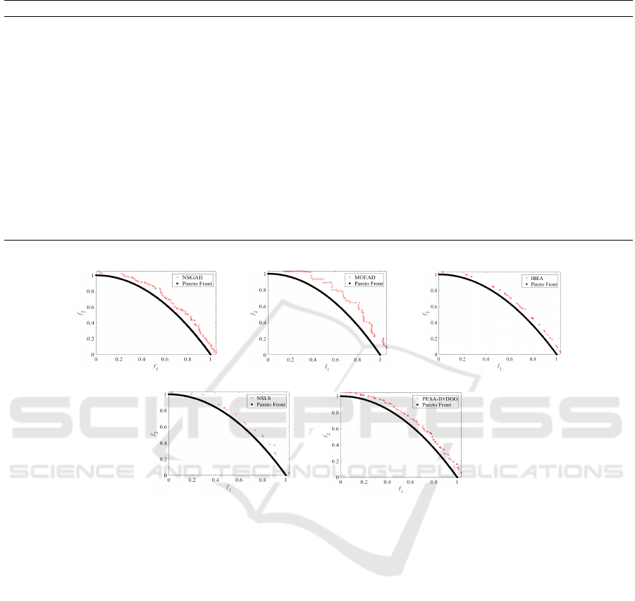
Table 5: Comparison results of the ﬁve algorithms on the UF and DTLZ test suites in term of IGD.

Problems NSGA-II MOED/D IBEA NSLS PESA-II+DGG

UF1

1.6537E−1(5.62E−2) 2.7100E−1(1.00E−1) 1.6278E−1(4.88E−2) 2.5520E−1(2.76E−2) 1.5827E−1(4.77E−2)

UF2

6.1831E−2(2.01E−2) 1.7084E−1(8.07E−2) 6.2608E−2(1.71E−2) 5.5395E−1(3.79E−2) 7.5380E−2(2.44E−2)

UF3

2.9459E−1(4.59E−2) 3.2462E−1(2.43E−2) 2.8530E−1(4.68E−2) 3.8590E−1(2.52E−3) 3.0581E−1(3.72E−2)

UF4

5.4031E−2(2.52E−3) 8.3697E−2(3.74E−3) 5.8447E−2(4.15E−3) 7.0373E−2(5.45E−3) 5.3647E−2(1.29E−3)

UF5

7.5661E−1(1.86E−1) 5.9337E−1(1.28E−1) 6.4726E−1(1.75E−1) 1.9925E+0(1.23E−1) 8.6005E−1(2.01E−1)

UF6

3.3181E−1(1.33E−1) 4.7767E−1(2.41E−1) 3.5317E−1(2.18E−1) 1.0892E+0(7.78E−2) 3.2328E−1(1.26E−1)

UF7

2.4500E−1(1.54E−1) 4.1291E−1(1.65E−1) 1.9426E−1(1.53E−1) 2.7945E−1(2.31E−2) 2.9626E−1(1.93E−1)

DTLZ1

3.1601E−1(2.30E−1) 2.0636E−2(7.14E−5) 1.6766E−1(1.00E−1) 2.9003E+1(3.10E+0) 1.9636E−2(1.59E−3)

DTLZ2

6.9104E−2(2.03E−3) 5.4464E−2(4.63E−7) 8.1858E−2(2.11E−3) 4.1622E−1(5.14E−2) 5.6004E−2(6.27E−3)

DTLZ3

3.1061E+0(1.93E+0) 5.9815E−2(4.36E−3) 2.7884E+0(2.41E+0) 1.6674E+2(141E+1) 1.3363E+0(1.20E+0)

DTLZ4

9.8091E−2(1.60E−1) 2.1377E−1(2.57E−1) 1.0997E−1(1.58E−1) 6.0497E−1(6.17E−2) 5.2816E−2(3.13E−3)

DTLZ5

5.6405E−3(3.15E−4) 3.3865E−2(3.13E−5) 1.6502E−2(1.69E−3) 3.7154E−1(5.20E−2) 4.3857E−3(2.79E−4)

DTLZ6

6.0003E−3(2.96E−4) 3.3911E−2(8.69E−6) 1.8060E−2(2.37E−3) 2.1798E−1(8.01E−2) 4.9680E−3(2.52E−4)

DTLZ7

8.5549E−2(4.99E−2) 1.9806E−1(1.64E−1) 9.7567E−2(7.63E−2) 5.0053E−1(6.03E−2) 4.4917E−2(1.74E−3)

(a) (b) (c)

(d) (e)

Figure 2: Approximations of PF

true

found by different algorithms on UF4: (a) NSGA-II, (b) MOEA/D, (c) IBEA, (d) NSLS

and (e) PESA-II+DGG.

produces the best results on four out of seven test

problems: DTLZ2, DTLZ3, DTLZ4 and DTLZ6 and

both MOPSO+DGG and MOPSO failed to converge

effectively on DTLZ1 and DTLZ7 test problems.

4.3 Comparisons with State-of-the-Art

Algorithms

To further demonstrate the performance of the pro-

posed strategy, we choose one integration algorithm

PESA-II+DGG to compare with four state-of-the-art

algorithms. Tables 5 gives the results of all the al-

gorithms on the UF and DTLZ test suites in terms

of IGD metric. Regarding UF test suite, PESA-

II+DGG plays best on three out of seven test prob-

lems: UF1, UF4 and UF6. IBEA attains the best

results on UF3 and UF7 while NSGA-II obtains the

best results on UF2 and MOEA/D achieves a bet-

ter value on UF5. Concerning the DTLZ test suite,

PESA-II+DGG strategy gets the best performance

on all the test problems except DTLZ2 and DTLZ3,

while MOEA/D yields the best results on DTLZ1 and

DTLZ3.

Table 6 shows the results in terms of HV on the

two test suites. About the UF test suite, PESA-

II+DGG strategy produces the best results on three

test problems: UF1, UF4 and UF6, with MOEA/D on

UF5, and with NSGA-II performs best on UF2, UF3

and UF7. For the DTLZ test suite, PESA-II+DGG

strategy performs best in three test problems includ-

ing DTLZ4, DTLZ5 and DTLZ7. MOEA/D gets the

best values on DTLZ1, DTLZ2 and DTLZ3, while

NSGA-II obtains the best results on DTLZ6.

To intuitively illustrate the results of different al-

gorithms, we plot their ﬁnal PF

approx

on UF4 and

A New Diversity Maintenance Strategy based on the Double Granularity Grid for Multiobjective Optimization

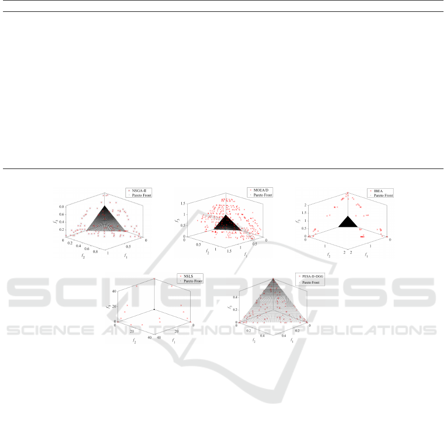
Table 6: Comparison results of the ﬁve algorithms on the UF and DTLZ test suites in term of HV .

Problems NSGA-II MOEA/D IBEA NSLS PESA-II+DGG

UF1

5.4521E−1(9.40E−2) 4.6001E−1(6.06E−2) 5.4568E−1(5.59E−2) 3.5544E−1(3.81E−2) 5.5198E−1(4.77E−2)

UF2

7.9102E−1(1.21E−2) 6.0930E−1(3.98E−2) 6.5537E−1(1.09E−2) 9.4796E−2(2.32E−2) 6.3947E−1(1.69E−2)

UF3

4.0706E−1(5.76E−2) 3.6294E−1(2.68E−2) 3.9449E−1(2.40E−2) 1.8994E−1(8.22E−3) 3.9866E−1(3.00E−2)

UF4

3.6256E−1(1.67E−2) 3.2340E−1(4.38E−3) 3.6811E−1(3.73E−3) 3.5117E−1(4.91E−3) 3.6973E−1(2.41E−3)

UF5

1.1454E−2(2.23E−2) 8.1769E−2(6.80E−2) 3.6548E−2(4.78E−2) 0.0000E+0(0.00E+0) 4.8915E−3(1.20E−2)

UF6

2.3175E−1(1.10E−1) 1.8840E−1(9.45E−2) 2.3286E−1(8.07E−2) 0.0000E+0(0.00E+0) 2.4.43E−1(6.96E−2)

UF7

4.4303E−1(1.19E−1) 2.6239E−1(1.06E−1) 4.0917E−1(1.01E−1) 1.6539E−1(3.51E−2) 3.4010E−1(1.19E−1)

DTLZ1

2.9097E−1(3.32E−1) 8.4082E−1(7.12E−4) 5.3077E−1(2.09E−1) 0.0000E+0(0.00E+0) 8.2774E−1(7.97E−3)

DTLZ2

5.3650E−1(3.53E−3) 5.5960E−1(6.44E−6) 5.5744E−1(1.19E−3) 4.6034E−2(3.80E−2) 5.4030E−1(7.32E−3)

DTLZ3

9.5069E−3(5.21E−2) 5.3461E−1(1.37E−2) 7.4213E−3(4.06E−2) 0.0000E+0(0.00E+0) 1.5676E−1(2.40E−1)

DTLZ4

5.2098E−1(8.15E−2) 4.8533E−1(1.23E−1) 5.4225E−1(8.53E−2) 0.0000E+0(0.00E+0) 5.4795E−1(6.81E−3)

DTLZ5

1.9853E−1(1.41E−4) 1.8188E−1(1.32E−5) 1.9869E−1(3.04E−4) 2.8943E−3(5.18E−3) 1.9916E−1(9.33E−4)

DTLZ6

1.9935E−1(1.43E−4) 1.8185E−1(4.19E−6) 1.9821E−1(4.39E−4) 1.2118E−1(1.77E−2) 1.9831E−1(1.98E−3)

DTLZ7

2.6915E−1(5.84E−3) 2.5216E−1(1.35E−2) 2.7431E−1(1.00E−2) 1.2069E−1(2.26E−2) 2.7853E−1(2.78E−3)

(a) (b) (c)

(d) (e)

Figure 3: Approximations of PF

true

found by different algorithms on UF4: (a) NSGA-II, (b) MOEA/D, (c) IBEA, (d) NSLS

and (e) PESA-II+DGG.

DTLZ1 test problems, in Fig. 2 and Fig. 3, respec-

tively. As can be seen from Fig. 2, the PF

approx

MOPSO-DGG is very close to the PF

true

and the

obtained nondominated solutions are uniformly dis-

tributed on PF

approx

, and the other four algorithms fail

to cover the PF

true

5 CONCLUSIONS

The diversity of nondominated solutions is a momen-

tous goal of evolutionary and swarm intelligence al-

gorithms for solving MOPs. The grid strategy is an

effective diversity maintenance strategy of nondomi-

nated solutions. However, the existing grid strategy

based on single-layer grid structure can not judge the

diversity of nondominated solutions in multiple hy-

perboxes with the same crowding degree. In this pa-

per, we proposed a new diversity maintainance strat-

egy based on the double granularity grid (DGG),

which obtains the more evenly distribution of non-

dominated solutions by dividing double granularity

grid. To demonstrate the performance of DGG strat-

egy, we integrated it with two popular algorithms

based on single-layer grid and compared it with four

state-of-the-art algorithms. The experimental results

show that the proposed DGG strategy is effective and

has great potential for maintaining the diversity of

nondominated solutions on MOPs problems.

In the future, we will further study the grid strat-

egy and develop a more effective diversity mainte-

nance strategy. Since the results of the proposed strat-

egy in many-objective optimization problem are not

very ideal, we also want to extend this strategy to the

many-objective optimization problem in the next step.

ICPRAM 2020 - 9th International Conference on Pattern Recognition Applications and Methods

ACKNOWLEDGEMENTS

This work is partly supported by the NSFC

Research Program (61672065, 61906010), Bei-

jing Municipal Education Research Plan Project

(KM202010005032), China Postdoctoral Science

Foundation funded project (71007011201801), Bei-

jing Postdoctoral Research Foundation (2017-ZZ-

024), and Chaoyang Postdoctoral Research Founda-

tion (2018ZZ-01-05).

REFERENCES

Aimin Zhou, Bo-Yang Qu, H. L. S.-Z. Z. and Zhang, Q.

(2011). Multiobjective evolutionary algorithms: A

survey of the state of the art. Swarm and Evolutionary

Computation, volume 1, pages 32–49.

Bili Chen, Wenhua Zeng, Y. L. and Zhang, D. (2015).

A new local search-based multiobjective optimization

algorithm. IEEE Transactions on Evolutionary Com-

putation, volume 19, pages 50–73.

Bosman, P. and Thierens, D. (2003). The balance between

proximity and diversity in multiobjective evolutionary

algorithms. IEEE Transactions on Evolutionary Com-

putation, volume 7, pages 174–188.

Coello, C. A., Pulido, G. T., and Lechuga, M. S. (2004).

Handling multiple objectives with particle swarm op-

timization. IEEE Transactions on Evolutionary Com-

putation, volume 8, pages 256–279.

Corne, D., Knowles, J., and Oates, M. (2000). The pareto-

envelope based selection algorithm for multiobjective

optimization. InInternational Conference on Parallel

Problem Solving from Nature, pages 869–878.

Corne D W, Jerram N R, K. J. D. e. a. (2001). PESA-II:

Region-based selection in evolutionary multiobjective

optimization. In GECCO’2001’ Proceedings of the

Genetic and Evolutionary Computation Conference,

pages 283–290.

Deb (2001). Multi-objective Optimization using Evoulu-

tionary Algorithms. Chichester, john wiley & sons

edition.

Deb (2014). Multi-objective Optimization, Search method-

ologies. Springer, Boston,MA.

E. Elejalde, L. Ferres, E. H. and Bollen, J. (2018). Quanti-

fying the ecological diversity and health of online

news. Journal of computational science, volume 27,

pages 218–226.

Eckart, Z. and K

unzli, S. (2004). Indicator-based selection

in multiobjective search. In in Proc. 8th International

Conference on Parallel Problem Solving from Nature

(PPSN VIII), pages 832–842. Springer.

Ge, H., Zhao, M., Sun, L., Wang, Z., Tan, G., Zhang, Q.,

and Chen, C. L. P. (2019). A many-objective evolu-

tionary algorithm with two interacting processes: Cas-

cade clustering and reference point incremental learn-

ing. IEEE Transactions on Evolutionary Computa-

tion, pages 1–1.

Huband, S., Barone, L., While, L., and Hingston, P. (2005).

A scalable multi-objective test problem toolkit. In

Evolutionary Multiobjective Optimization,Springer.

JD, K. and DW, C. (2000). Approximating the non-

dominated front using the pareto archived evoluton

strategy. IEEE Transactions on Evolutionary Com-

putation, volume 8, pages 149–172.

K. Deb, L. Thiele, M. L. and Zitzler, E. (2005). Scal-

able test problems for evolutionary multiobjective op-

timization. IEEE Transactions on Evolutionary Com-

putation, volume 20, pages 105–145. Springer.

K. Deb, A. Samir, P. A. and Meyarivan, T. (2000). A fast

elitist non-dominated sorting genetic algorithm for

multi-objective optimization: NSGA-II. IEEE Trans-

actions on Evolutionary Computation, pages 849–

858. Springer.

Li, M., Yang, S., and Liu, X. (2014). Shift-based den-

sity estimation for pareto-based algorithms in many-

objective optimization. IEEE Transactions on Evolu-

tionary Computation, volume 18, pages 348–365.

Margarita, R. and Coello, C. C. A. (2006). Multi-objective

particle swarm optimizers: A survey of the state-of-

the-art. International journal of computational in-

teligence research, volume 2, pages 287–308.

X. Cai, Z. F. and Zhang, Q. (2017). A conatrained decom-

position approach with grids for evolutionary multi-

objective optimization. IEEE Transactions on Evolu-

tionary Computation, volume 22, pages 564–557.

Yang, Shengxiang, L. M., Xiaohui, L., and Jinhua, Z.

(2013). A grid-based evolutionary algorithm for

many-objective optimization. IEEE Transactions on

Evolutionary Computation, volume 17, pages 721–

736.

Z. Eckart, K. J. and Lothar, T. (2008). Quality assessment

of pareto set approximations. In Evolutionary Mul-

tiobjective Optimization, volume 52, pages 373–404.

Springer.

Zhang, Q. and Li, H. (2007). MOEA/D: A multiobjec-

tive evolutionary algorithm based on decomposition.

In IEEE Transactions on Evolutionary Computation,

volume 11, pages 712–731.

A New Diversity Maintenance Strategy based on the Double Granularity Grid for Multiobjective Optimization