
Comparison of Algorithms for Tree-top Detection
in Drone Image Mosaics of Japanese Mixed Forests
Yago Diez
1 a
, Sarah Kentsch
2 b
, Maximo Larry Lopez Caceres
2 c
, Ha Trang Nguyen
2
,
Daniel Serrano
3
and Ferran Roure
3 d
1
Faculty of Science, Yamagata University, Japan
2
Faculty of Agriculture, Yamagata University, Japan
3
Eurecat, Technology Centre of Catalonia, Spain
Keywords:
Computer Vision, Tree Detection, Mixed Forests, Clustering Techniques.
Abstract:
Counting trees is a common problem in forest applications often solved by performing field studies that are
exceedingly cost-intensive in time and manpower. Consequently, many researchers have used computer vi-
sion techniques to automatically detect trees by finding tree tops. The success of these algorithms is highly
dependent on the data that they are used on. We present a study using data acquired by ourselves in a natural
mixed forest using an Unmanned Aerial Vehicle (UAV). Given the particularly challenging nature of our data,
we developed a pre-processing step aimed at preparing the data so that it could be used with six common
clustering algorithms to detect tree tops. Extensive experiments using data covering over 40 ha is presented
and tree detection accuracy, tree counting metrics and computation and use time considerations are taken into
account. Our algorithms detect over 80% with high location accuracy and up to 90% with lower accuracy.
Tree counting errors range from 8% to 14% for most methods. Data Acquisition and runtime considerations
show how this techniques are ready to have an immediate impact in the processing of real forest data.
1 INTRODUCTION
Forests occupy approximately 68 % of the total ter-
ritory of Japan. Most of these are deciduous mixed
forests (Shimada, 2009), an ecologically complex va-
riety due to the changing distribution of tree species
within a stand or the many inter-species interactions.
Nowadays, the research on these issues is carried out
using land surveys which are labor-intensive, expen-
sive and some times dangerous for human surveyors.
In order to maintain the Japanese forest ecosystem
it is necessary to gain a deeper understanding about
how the different species interact and are distributed.
Thus, we need to develop methods to gather and pro-
cess information from these forests in a way that is
fast, efficient and reliable.
Unmanned Aerial Vehicles (UAVs) are rapidly be-
coming an essential tool in agriculture (Grenzd
¨
orffer
and Teichert, 2008; Honkavaara et al., 2013; Raparelli
a
https://orcid.org/0000-0003-4521-9113
b
https://orcid.org/0000-0001-5693-5217
c
https://orcid.org/0000-0002-9748-7120
d
https://orcid.org/0000-0003-1005-4267
and Bajocco, 2019) and forestry applications (Tang
and Shao, 2015; Paneque-G
´
alvez et al., 2014; Ad
˜
ao
et al., 2017; Grenzd
¨
orffer and Teichert, 2008; Gam-
bella et al., 2016). UAVs represent an easy-to-use, in-
expensive tool for remote sensing of forests because
they can fly close to tree canopies resulting in im-
proved image resolution (pixels representing a few
centimeters as opposed to several meters in satellite
imagery (Onishi and Ise, 2018)).
On the other hand, computer vision techniques
have long been used in a variety of areas ranging
from 3D reconstruction (Roure et al., 2019) to medi-
cal imaging (Garc
´
ıa et al., 2019). Lately, the increase
in data availability and the apparition of new tech-
niques such as Deep Learning has further increased
the research areas where some well established com-
puter vision concepts such as segmentation, registra-
tion or classification are used. These new areas range
from research field so apparently distant as document
processing (Diez. et al., 2019) or forestry (Onishi and
Ise, 2018).Among all the computer vision algorithms
techniques usable with the high-resolution images ob-
tained by drones, we are interested in those that help
as solve the problem of detecting individual trees.
Diez, Y., Kentsch, S., Caceres, M., Nguyen, H., Serrano, D. and Roure, F.
Comparison of Algorithms for Tree-top Detection in Drone Image Mosaics of Japanese Mixed Forests.
DOI: 10.5220/0009165800750087
In Proceedings of the 9th International Conference on Pattern Recognition Applications and Methods (ICPRAM 2020), pages 75-87
ISBN: 978-989-758-397-1; ISSN: 2184-4313
Copyright
c
2022 by SCITEPRESS – Science and Technology Publications, Lda. All rights reserved
75

In agriculture, tree counting is a common tech-
nique for getting accurate information about tree
stands (Pont et al., 2015; Bazi et al., 2014; Santoro
et al., 2013). Also in forestry, finding individual trees
is necessary for tasks such as tree height and carbon
stock estimations, tree classification (Natesan et al.,
2019; Onishi and Ise, 2018) and even high-level tasks
in forest management and field survey (Richardson
and Moskal, 2011; Korpela et al., 2007). However,
factors like the variability of individual trees (size,
species), soil background signal and man-made ob-
jects present challenges for image analysis algorithms
(Santoro et al., 2013). As a result most of the existing
studies are carried out in plantations, where these fac-
tors are minimised (Jusoff, 2009; Shafri et al., 2011;
Gougeon and Leckie, 2006).
In this paper we adapt and apply six well known
clustering and extrema detection computer vision al-
gorithms to the detection of tree tops in dense and un-
managed forests. We present a comprehensive study
of the different algorithms including analysing the
correctness, precision and speed of each strategy.
The rest of the paper is organised as follows. Sec-
tion 2 discusses previous work in computer vision for
tree detection and counting. Section 3 formally de-
fines the problem and provides details on the data ac-
quisition process. Given the considerations made in
the previous section, we also present extensive dis-
cussion on the characteristics of the data and how
they affect our study. Section 4 provides details on
the algorithms used to detect tree tops and the pre-
processing and post-processing steps that we devised
to overcome some of the difficulties posed by the data.
Section 5 provides quantitative evaluation of the re-
sults obtained. The paper end with the conclusions
and considerations on future work in Section 6.
2 STATE OF ART
Tree counting techniques are useful to provide infor-
mation for management and economical issues, es-
pecially in agricultural and forest plantations (Shafri
et al., 2011; Mubin et al., 2019; Hossein Mojad-
dadi Rizeei and Kalantar, 2018; Aliero et al., 2014;
Weinstein et al., 2019). Therefore, the detection of
single trees under influencing factors like stand age
and height, dominance of tree species in a stand,
topography and illumination conditions are of eco-
nomic importance (Hirschmugl et al., 2007). Ini-
tial studies proposed the use of the high reflectance
of tree tops in comparison to the surrounding pix-
els of the tree crown (Pinz, 1989; Gougeon, 1995;
Pitk
¨
anen, 2001; Pouliot et al., 2002). These meth-
ods were followed by approaches using Watershed
segmentation and Region Growing to delimit tree
crowns once an initial set of tree tops had been de-
termined (Ke and Quackenbush, 2011). Local ex-
trema, and morphological operators where also used
to increase the detectability of trees (Ke and Quack-
enbush, 2011). (Erikson and Olofsson, 2005) used
points with high grey value as seed regions and then
compared the Region Growing, Template matching
and Brownian motion methods to delineate the tree
crowns. (Hirschmugl et al., 2007) used a Digital El-
evation model DEM to detect seed regions of single
trees in their images. These DEM images are images
with the same dimensions of the data but where every
pixel represents altitude information. Their approach
was based on a comparison between 2d morph algo-
rithm and a 3d-block-based model in order to detect
tree tops in a dense natural mixed forest from a non-
alpine area. The authors were able to detect 64% with
the 2D approach and 70% with the 3D one. In a fur-
ther step they combined the seed detection with the
Region Growing algorithm, a local maxima approach
and a morphological operator to improve the accuracy
of the detection. (Larsen et al., 2011) proposed that
all algorithms can be successful under special condi-
tions by comparing different algorithms on different
datasets and forest conditions.
Latest studies combined high resolution imagery
and deep learning approaches to derive high quality
forest information (Li et al., 2017; Mubin et al., 2019;
Weinstein et al., 2019; Csillik et al., 2018). (Li et al.,
2017) introduced the first detection method using a
Convolutional Neural Network (CNN) for counting
oil palm trees which were characterized as crowded
and with a high overlap of the trees. The study
used RGB satellite images. First, a CNN model was
trained to classify the data into tree and background
classes. Then, a sliding window technique with pixel
merging was used to increase the detection of trees.
An accuracy of 96% compared to the ground truth
data was achieved using independently collected im-
ages. (Mubin et al., 2019) where able to separate
young and mature oil palm trees by using two CNNs.
with accuracy reaching 95%. (D
´
ıaz-Varela et al.,
2015) took up the approach of using the DEM. They
performed flights with an UAV and used geographical
information system analyses, as well as object-based
classifications to detect the trees and estimate their
height and crown diameter. (Torres-S
´
anchez et al.,
2015) conducted successfully UAV flights, genera-
tions of DEM and object-based image analysis tech-
niques. RGB, multispectral images and DSMs were
used to segment olive trees in a plantation. The DSM
was used to eliminate non-olive vegetation. Multi-
ICPRAM 2020 - 9th International Conference on Pattern Recognition Applications and Methods
76

spectral images provide the best results with an over-
all accuracy of up to 97%.
Most of the mentioned studies have been con-
ducted in plantations and achieved high accuracy in
tree detection. However, as pointed out in (Larsen
et al., 2011), most algorithms are highly dependent
on the data they are used with. The conditions in
mature forests, like shadowing, reflectance variations
within the crown or overlapping branches make them
a very challenging scenario. Methods like Region
Growing are sensitive to reflectance, while the valley-
following algorithm reaches its limits by recogniz-
ing single trees in a dense forest (Ke and Quacken-
bush, 2011). Also, (Li et al., 2017) pointed out that
problems occur with small and young trees by using
maximum filtering, as well as problems with template
matching when tree stands are too crowded. Natu-
ral (non-plantation) forests, present further difficulties
as mixed species in forests, separating trees from the
underground vegetation and varying density of trees
(Skurikhin et al., 2013). The first step of all the algo-
rithms mentioned in this section is the detection of
trees. Therefore, in this paper focus on this issue.
Specifically we address the issue of detecting tree tops
by using mosaics and DEM in an exceedingly chal-
lenging scenario due to our forests being natural, un-
managed, mixed and set in areas with steep slopes.
3 DATA USED
Most natural mixed forests in Japan are located in
mountain areas. As a part of the northern most area of
the Asahi Mountains, our study field is a representa-
tive mixed forest for Japan. Research sites cover areas
close to the river up to the ridges in a height of more
than 2000 m. The mean slope angle of the mountain’s
ranges between 33 and 40 % (Lopez et al., 2014). The
dense structure and the high under-storey vegetation
are characteristics for this forest. In this area we are
able to determine dominate tree species, but a specific
statement about all tree species, their locations and
number is not possible.
3.1 Data Acquisition
Data acquisition was carried with a DJI Phantom 4
and a DJI Mavic 2 Pro. Both are small and user-
friendly drones which are able to cover different sites
for image collection. The drones are equipped with
a 12 megapixel (Phantom) and 20 megapixel camera
(Mavic) taking high resolution images. The cameras
collect RGB images. Both drones are using GPS and
GLONASS satellite systems to georeferenced the po-
sition of the drone. Pre-programmed flights are done
with the app DJI GS Pro, which standardize the flight
protocol. The flight time ranges between 15 min up
to 30 min depending on the cover area of the sites.
Locations. Taking into account the diversity of
forests in Japan we decided to select two locations
representing different forest environments (see Figure
1). The first location is the Yamagata University Re-
search Forest (YURF) located on the main island of
Japan, Honshu. This mixed natural forest is part of
the Ashahi mountain, covers an area of 753,02 ha and
is characterized by steep slopes and river areas. Im-
age collection was done in different sites of the for-
est. Seven flights were carried out at the beginning
of summer season 2019. The cover area varies be-
tween 3 and 6 ha. Four sites are located close to a
river, while four others are located in the slope of the
mountains. Therefore, flight altitudes between 80 and
140 m and an overlap between 90 and 96 % were cho-
sen. The number of raw images was between 214 and
418 per site.
The second study site is the Zao mountain, a vol-
cano in the southeastern part of Yamagata Prefecture.
The mountain is mostly composed of fir trees (Abies
sachalensis) affected by moth and bark beetle infes-
tations. The study sites are located at different al-
titudes of the mountain characterized by sites with
steep slopes and flat areas. Image collection took
place during the summer season 2019. Three sites
were imaged with a flight altitude between 60 and 70
m. The cover area ranges between 2.9 and 12.7 ha and
up to 495 images were collected in one flight.
3.2 Data Processing and Annotation
The collected raw images were processed by
Metashape. This software uses the image informa-
tion to align the pictures of each flight to generate a
dense point cloud. The dense cloud is used to create a
mosaic. Furthermore, the software generates a Digi-
tal Elevation Model (DEM), which is also used in this
approach. The mosaic contains colour information,
while in the the DEM shows the different elevations
in a gray-scale format. Examples of the mosaics can
be seen in figure 1 (right) while the center part of the
same figure contains examples of DEMs. In total, a
number of 10 mosaics, as well as their DEMs were
considered for this study.
The next step that we followed was the annota-
tion process. This was done manually using an image
manipulation software. We used the mosaic and the
DEM as single layers and added a third layer for the
annotations. Higher spots were marked with a black
dot in the third layer on the basis of the DEM. The
Comparison of Algorithms for Tree-top Detection in Drone Image Mosaics of Japanese Mixed Forests
77
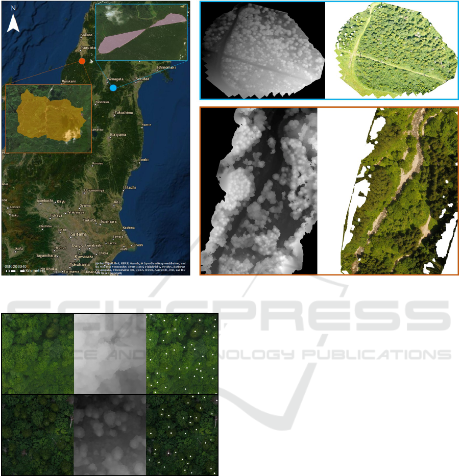
Figure 1: Location of Data acquisition sites (left) and two examples of the data used for tree top detection, DEMs (center) and
mosaics (right).
Figure 2: Detail of the mosaic data (left), the mosaics (cen-
ter) and the results of annotation (right), tree tops are pre-
sented as white points.
mosaic was used to confirm, that the high points visi-
ble in the DEM belongs to tree tops. Figure 2 presents
a part of one of the mosaics with superimposed anno-
tation data.
3.3 Challenges in Data and Limitations
of this Study
As mentioned in section 2, some previous approaches
tried to solve the problem of tree counting using
the visual information of the RGB photogrametry
(Hern
´
andez Hern
´
andez et al., 2016). I.e., in agri-
culture, the trees can be detected using computer vi-
sion techniques like thresholding or contour detec-
tion. This task becomes possible due to the colour
differences between ground and trees that can be ob-
served in the fields. This is made easier by trees being
planted in a way that facilitates the access to agricul-
tural machinery. In other scenarios, like unmanaged
forest, where trees grow without a pre-determined
pattern, tree detection becomes much more difficult.
The main problem in this kind of landscape is that the
trees grow very close to each other and it is impos-
sible to identify which part of crown belongs to one
tree or another. For this reason, a 3D reconstruction
of the forest, expressed through a DEM that contains
the height information at each pixel, becomes a very
useful tool. Identifying the local highest points in the
DEM would then give us a tree count of the examined
area. However, more difficulties arise. One important
problem is the variability of the tree distribution in a
single scenario.
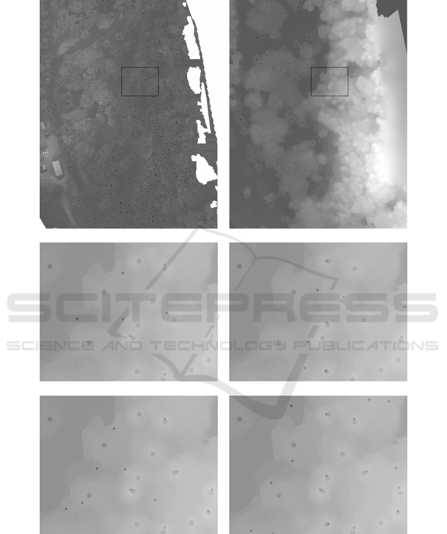
Figure 3 (top left and center right) shows an ex-
ample of this variability, where an area covered by
a high number of trees is next to another area with
only few isolated trees. This forces to use adaptive
algorithms to not loss any tree top. Another impor-
tant challenge is the heterogeneous terrain with steep
ICPRAM 2020 - 9th International Conference on Pattern Recognition Applications and Methods
78
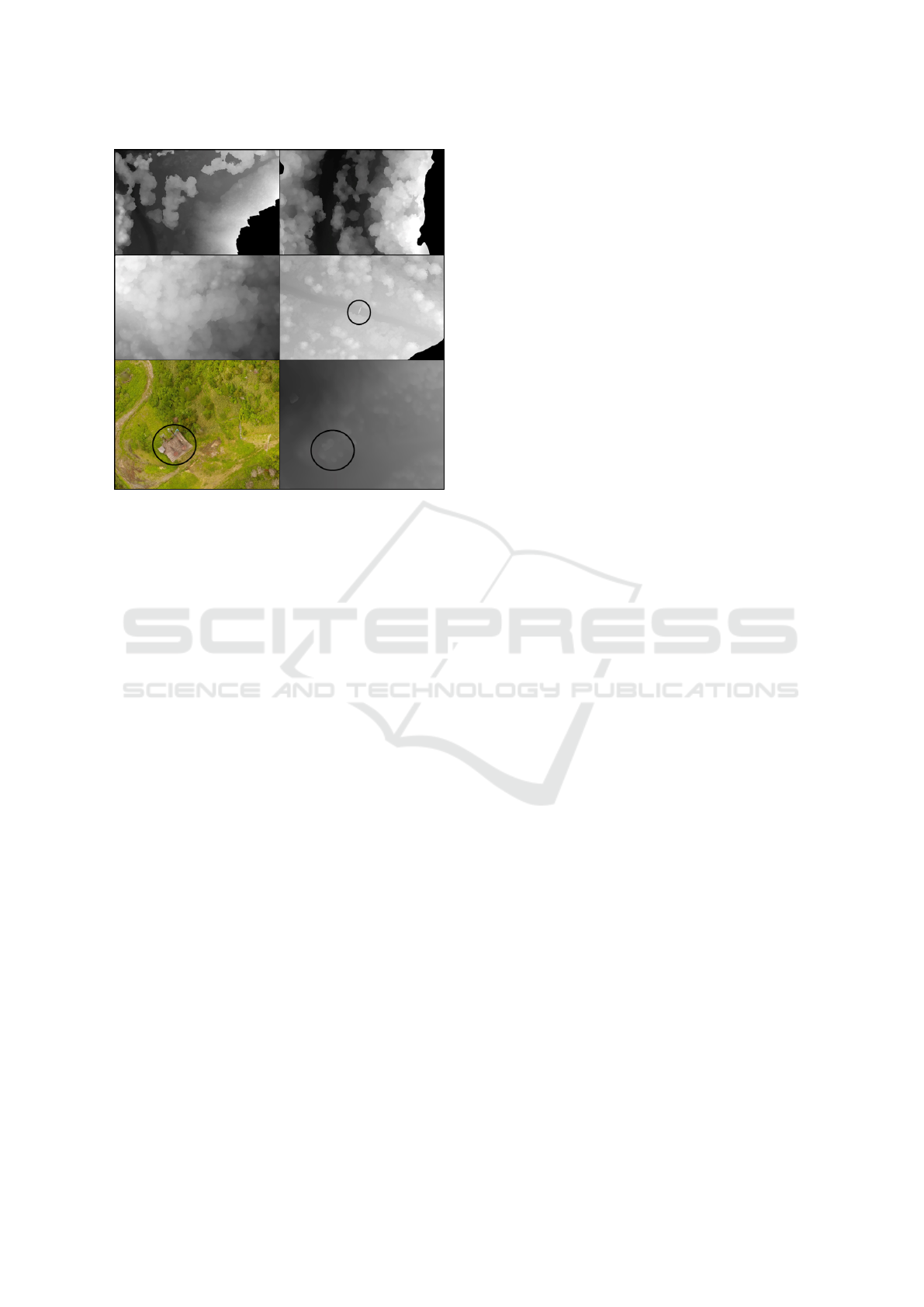
Figure 3: Difficulties in data. Top Left show a DEM with a
slope with bushed but no trees. Top Right and Center Left,
details of two DEMs showing a large degree of variation of
tree density, within the same DEM and from one DEM to
another. Center Right and Bottom, show distortion caused
by man-made objects. Center Right contains an electricity
tower while Bottom Right shows how the building high-
lighted in Bottom Left appears in the DEM.
slopes. As lighter pixels represent higher altitudes” it
is important to bear in mind that each value contains
both the altitude of the floor plus the altitude of any
tree that the pixel may belong to. Consequently, the
tree detection algorithms should look for altitude val-
ues that are local maxima but only in those regions
containing trees. For example, in some uphill parts
of the forest the floor itself may be higher than trees
present in the same mosaic with or without contain-
ing trees (Figure 3 top right). Finally, other issues
may represent problems for our algorithms: artefacts
produced by the mosaic computation, where corners
can be distorted due to a lack of images or the pres-
ence of man-made objects such as electricity towers
(Figure 3 center right) or buildings (Figure 3 bottom).
Taking all of this into account, we reviewed the 10
mosaics collected. In 2 of them we considered that the
conditions, mostly concerning tree density, were too
different from the other eight sites. The algorithms
were able to compensate a certain degree of tree den-
sity variability which leaded to good results for those
two. Anyway, it was not possible to obtain good re-
sults with a single set of parameters for all of the 10
DEMs at the same time. Consequently, we discarded
these two DEMs and focused the study on the remain-
ing 8.
4 MATERIAL AND METHODS
4.1 Tree Top Detection Algorithm
In this section we present the algorithms used to ex-
tract tree tops from our DEM images. We started by
collecting the data and annotating manually where the
tree tops were located. In order to achieve algorithms
that automatically retrieved the same tree top infor-
mation we initially expected that we would have to
make the algorithms search for local DEM pixel in-
tensity maxima (as was, for example, mentioned in
(Natesan et al., 2019)). However, we soon realised
that our data presented additional challenges. Specif-
ically, we observed that the numbers of tree candidate
points outside of the regions properly containing trees
was very high. This happened mainly because the up-
hill disposition of the forests detailed in section 3.3.
Tree tops where often not local DEM maxima (in the
case when the plot was close to an uphill section of
the area) and there were regions at different altitude
values (sometimes including the DEM global maxi-
mum) that did not contain trees.
Moreover, the density of trees was very irregular.
For example, within the same mosaic, three windows
of the same size were observed to contain 10, 4 or
2 tree tops in different parts of the forest captured in
different DEMs. Even inside the same DEM, this tree
density varied significantly, even discounting the ar-
eas not containing any trees. This made running the
tree detection algorithms with the same set of param-
eters for the whole of each mosaic impractical.
In order to reduce the impact of these issues, we
preceded the algorithms aimed at detection tree tops
with a pre-processing algorithm that had the follow-
ing goals: First of all, remove the part of the DEM
that clearly corresponded to the lower floor area (that
is, the lower floor part not belonging to uphill parts of
the site). Then, highlight the highest part of the image
in the cases where it was possible to isolate a set of al-
titudes not containing any (uphill) floor section. And,
finally, provide a map of the sections of the DEM con-
taining sudden variations in altitude between a pixel
and its neighbors.
This resulted in an ”interest map” (see Section
4.1.1 for details). Afterwards, a tree top detection
algorithm among six previously existing algorithms
was run in the DEM taking into account the informa-
tion encoded in the interest map.
4.1.1 Interest Region Extraction
This strategy is divided in three parts. First the DEM
was divided in interest regions according to height
Comparison of Algorithms for Tree-top Detection in Drone Image Mosaics of Japanese Mixed Forests
79
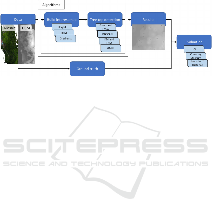
Figure 4: Overview of the Algorithms studied in this paper.
associated to each pixel, then it is divided into re-
gions associated to the presence or absence of large
DEM intensity gradients. Finally, the two divisions
are combined to create an interest map of the DEM.
In the first step, a simple absolute thresholding al-
gorithms was used to assign to each pixel in the DEM
a label in terms of its height: A value of 0 was as-
signed to pixels belonging to the floor. To be precise,
this meant the lowest part of the floor that could be
discarded as not containing any trees. Floor sections
in the uphill part of the sites were not discarded by this
step. Pixels not belonging to this ”floor” part were as-
signed a value of 2 if the higher values in the DEM
were seen to belong to treetops. In some mosaics no
pixels received this value. Pixels not clearly identified
as floor or tree tops by thresholding where assigned a
value of 1.
In the second step of the algorithm, each pixel was
assigned a value according to whether or not it has
large DEM gradients nearby. A value of 0 meant that
the pixel did not have those gradients nearby while a
value of 2 meant that it did. In order to do this the
Sobel filter (Danielsson and Seger, 1990) was used to
find large gradients both in the x and y direction. A
gradient image was built for each direction and both
were added into a single gradient image. However,
the DEM gradients tend to show in the borders of the
tree crowns as the differences between the lower part
of the tree crown is where sudden differences in al-
titude are easier to observe. As our goal was to find
tree top points that were enclosed inside of the tree
crowns thus outlined, we used a morphological clos-
ing operator (Haralick and Shapiro, 1992) in order to
obtain the enclosed regions.
Finally, the two sets of labels were combined:
• 0 −→ Pixel belongs to the floor not in any uphill
section.
• 1 −→ Not floor,not high, no gradients.
• 2 −→ High pixel, no gradients.
• 3 −→ Not floor not high, Gradients present.
• 4 −→ High Pixel with gradients.
Figure 5 shows an example of an interest map. Notice
in the detail subfigure how regions with higher tree
top density are marked as higher interest with brighter
pixel intensity. The difficulty of the terrain can be
observed in the bottom left corner of the main figure.
A narrow section marked as high interest contains no
trees. This happens because this section is situated in
an uphill part of the site with an altitude close to that
of the higher tree tops and containing low bushes that
presented detectable gradients.
4.1.2 DEM Sliding Window Clustering
After building the interest maps, several algorithms
were used for tree top detection. In all of them, and
following previous approaches such as, for example
(Natesan et al., 2019), a sliding window approach was
used. The size of this window was one of the param-
eters that affected the performance of the algorithm
the most. For each position of the window, one of six
possible tree top detection algorithms was computed.
Iterative Global Maxima. The iterative Global Max-
ima (GMax) algorithm consists on finding only the
maximum intensity value in each window. This ap-
proach is highly dependant on the window size, be-
cause some trees can be discarded if the window is
too big due to only the highest value on the window
will be picked. Nevertheless, this is one of the sim-
plest and less time consuming algorithms.
Peak Local Maxima. This algorithm, referred to
from now on as LMax, looked for several DEM in-
tensity local maxima in each window. This algo-
rithm was used in (Natesan et al., 2019) although no
detailed results were reported as the work there fo-
cused on tree classification. The algorithm first used
ICPRAM 2020 - 9th International Conference on Pattern Recognition Applications and Methods
80
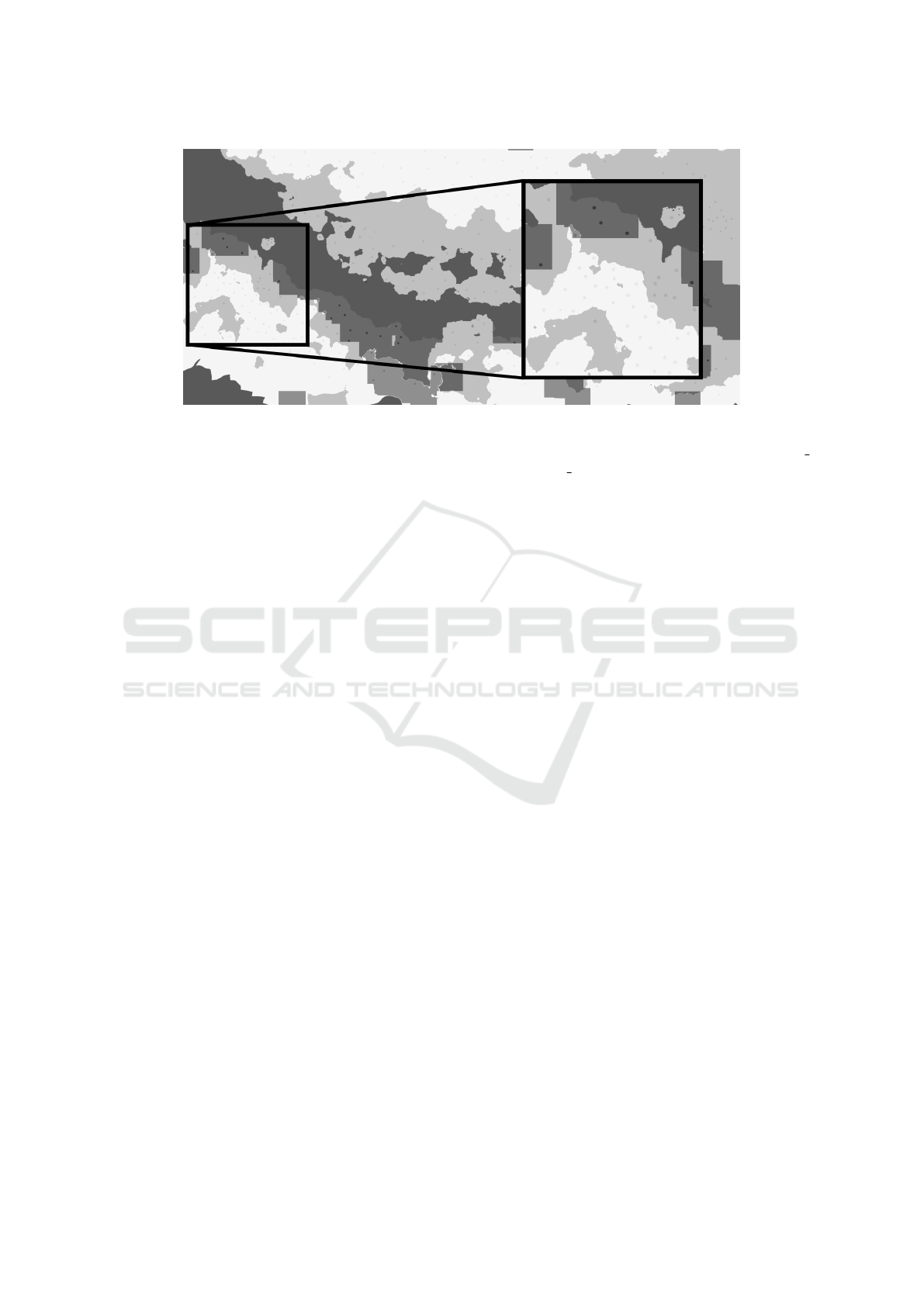
Figure 5: Interest Map example with superimposed tree tops as points.
a gaussian smoothing over the altitude values and
those under a certain threshold were discarded. Then
only maxima that were too close to another maxi-
mum were discarded. This was done using two pa-
rameters, th for the blurred DEM thresholding and
md for the minimum distance between maxima. We
used the implementation of the algorithm that is pub-
licly available at: https://scikit-image.org/docs/0.7.0/
api/skimage.feature.peak.html.
DBSCAN. DBSCAN stands for ”Density based spa-
tial clustering”(Ester et al., 1996). This is a cluster-
ing algorithm tha takes the density of data into ac-
count. The algorithm groups nearby points using a
parameter ε and then marks points not grouped as
outliers. The implementation that we used, publicly
available at https://scikit-learn.org/stable/modules/
generated/sklearn.cluster.DBSCAN.html, also con-
tains a parameter ms to filter cluster centers that are
too close to each other.
K-Means. K-Means, referred to form now on as KM
is a well-known clustering algorithm (Lloyd, 1982).
The algorithm partitions the data k clusters. Each
pixel belongs to the cluster with the mean intensity
closer to its own intensity value. The specific algo-
rithm used for this as well as the subsequent cluster-
ing algorithm is the number of classes considered nc.
The implementation used for this study is available
at: https://scikit-learn.org/stable/modules/generated/
sklearn.cluster.KMeans.html
Fuzzy C-Means. Fuzzy C-Means (FCM) is a vari-
ation of the K-Means algorithms that assigns, for
each pixel a probability to belong to each existing
cluster (Bezdek et al., 1984). Centroids for every
cluster are computed taking into account the prob-
ability of each pixel to belong to the cluster and a
fuzziness parameter that changes the weight of the
contribution of each pixel. In our use of this al-
gorithm we started from the implementation avail-
able at: https://pythonhosted.org/scikit-fuzzy/auto
examples/plot cmeans.html, considered the nc pa-
rameters and set a fixed fuzziness value.
Gaussian Mixture Model. The Gaussian Mixture
Model GMM algorithm for clustering data considers
every cluster as a normal (or Gaussian) random vari-
able. At each step of the algorithm the probability of
every pixel to belong to every cluster (or Gaussian)
is computed. The parameter defining the Gaussian
functions associated to each cluster are then updated
using an expectation maximization algorithm. The al-
gorithm ends when a certain convergence criterion is
held. In our case we have used the same nc parame-
ter representing the number of clusters as in the two
previous algorithms. We have used the following im-
plementation: https://scikit-learn.org/stable/modules/
mixture.html .
4.1.3 Use of Interest Maps to Refine the
Detected Tree Tops
For all algorithms, any tree top detected in the section
labelled 0, was discarded. For all of the other sec-
tions, tree tops were assigned an ”uncertainty” region
in the shape of a disk of varying radius. Then inter-
secting uncertainty reasons were merged and a single
representative tree top was used. The interest map
was used to make the uncertainty regions in lower in-
terest regions have larger radii. With this, the number
of points in lower interest regions was reduced.
For the three parameterised clustering algorithms
(KM, FCM,GMM), the average of the interest map
labels of the pixels in each window was used to ad-
just the number of clusters being detected with higher
interest regions being assigned more clusters.
Comparison of Algorithms for Tree-top Detection in Drone Image Mosaics of Japanese Mixed Forests
81

5 EXPERIMENTS
All the algorithms described throughout the paper
were implemented using the python programming
language (Van Rossum and Drake Jr, 1995). General
image manipulation was performed using the opencv
library (Bradski, 2000) while the scikit-learn library
(Pedregosa et al., 2011) was used to implement the
clustering algorithms. All experiments were run in a
workstation using a Linux Ubuntu operating system
with 10 dual-core 3GHz processors and an NVIDIA
GTX 1080 graphics card.
Parameter Tuning:
The ultimate goal of our current work is to produce
algorithms that can be used in practical settings to ex-
tract information from forest mosaics. In this context,
users are not expected to be able to fine-tune complex
computer vision algorithms. Moreover, as mentioned
in section 3.3, the DEM and mosaics used for this ex-
periments were determined to have similar character-
istics of tree density. On the other hand, the algo-
rithms presented have many parameters to configure
that result in wildly varying performances. Best re-
sults in terms of the evaluation metrics are obtained
by painstakingly testing out parameter combinations
for each DEM image.
Bearing these two issues in mind, in this sec-
tion we have limited ourselves to reporting, for each
method, the best results obtained on average over all
tested DEMs over one single set of parameters. That
being said, we performed extensive testing with as
many as 500 combinations of parameters for each
method in order to obtain the best possible parameter
combination. In terms of the use of the algorithms,
this can be seen as an offline ”set up” step for the sys-
tem that can then used as a black box by the users.
5.1 Quantitative Evaluation
In this section we report the performance of the six
methods studied in terms of three objective measures:
Hausdorff Distance:
d
H
(A, B) = max
sup
a ∈ A
in f
b ∈ B
d(a, b),
sup
b ∈ B
in f
a ∈ A
d(a, b)
The Hausdorff distance represents a convenient
way to measure distance between point sets. This
will allow us to conveniently compare the overall
performance of all the studied methods. This metric,
however, is somewhat abstract and vulnerable to
outlier points skewing the value. Consequently, we
provide two other metrics, aimed at addressing issues
of practical interest.
Matched Ground Truth Points Percentage (m%):
The first one, the percentage of ground truth points
matched gives us an indication of what percentage
of the tree tops were detected. In order to do this,
we considered a value that roughly represented the
radius of a tree crown and considered points matched
if they were within this threshold of each other. This
addresses the issue of whether the points detected
are placed in the right place. However, during our
experiments we realised that methods simply pro-
viding a large number of candidate points obtained
values for this metric that did not agree with our
subjective evaluation of their performance. Thus, in
order to complement this metric, we provide a simple
metric based on the difference between the number of
ground truth points and the number of detected points.
Counting Measure:
Stands for the difference of the trees present in the
mosaic ”n”, with the number of tree tops detected ”d”
weighted over the number of trees cnt =
n−d
n
. Con-
sequently, negative values indicate that the algorithm
underestimated the number of trees while positive val-
ues indicate overestimation. When we report averages
we have taken the absolute value of each value to pre-
vent these two errors cancelling each other.
Only methods achieving good results for the three
metrics at the same time (as low as possible for Haus-
dorff and cnt and as close to 100 as possible for m%)
are reported.
5.2 Results
Figure 6 and Table 1 present quantitative results for
this experiment. An example of the data used as well
as result for some of the methods can be found in
Figure 7. Figure 6 presents the average Hausdorff
distance, over all 8 mosaics considered, for the six
methods studied. Best results are obtained by GMM
(1170.26), DBSCAN (1194.10) and KM (1198.85).
GMax and FCM obtain results close to 1250 while
the result of LMax is over 1440. This indicates a su-
perior performance in terms of this distance of clus-
tering methods over those aimed at finding intensity
maxima.
Table 1 presents results for the cnt and m% mea-
sures for each method and DEM. The table is divided
into two parts, the top part contains information about
five of the DEMs while the lower part contains infor-
mation on the remaining three as well as the average.
Each row corresponds to one method and each pair of
columns to the performances of all the studied meth-
ods for one particular DEM. The final two columns
contain the averages of the cnt and m% measures. No-
tice that positive cnt values indicate that the algorithm
ICPRAM 2020 - 9th International Conference on Pattern Recognition Applications and Methods
82

Figure 6: Average Hausdorff Distance values over all DEM
images for the six methods studied.
overestimated the number of trees, negative values in-
dicate underestimation and that the average presented
was computed using average values so as not to can-
cel both errors out.
In this case, best results are observed for the
GMax algorithm achieving the best matched point
percentage and counting measure (90.64 , 8.09). High
results of over 80% on matching percentage were ob-
tained by FCM (81.88, 13.15), GMM (81.15, 14.25)
AND DBSCAN (80.94, 14.28). KM is able to match
slightly fewer tree tops but is better at counting them
(76.90, 11.50) while LMax obtains the worst results
with still high matched tree percentage but a clear ten-
dency to overestimate the number of trees producing
a bad cnt value (72.47, 27.49).
Table 1 and Figure 6 seem to be painting a slightly
different picture concerning method performance. We
believe the main reason for this has to with the be-
haviour of algorithms in areas of extreme point tree
top density. That is, areas with very few or many tree
tops. On the one hand, the GMax algorithm tends
to place a similar number of points in all these areas
(this behaviour is corrected to a certain extent by the
use of interest maps detailed in section 4.1.3). Con-
versely, algorithms such as GMM and FCM tend to
place fewer points than Gmax in lower density areas
and more in higher density areas. The extra points
in lower density areas heavily penalise the Hausdorff
value for GMax while the extra points in high den-
sity areas penalise a little bit the counting measure
for clustering methods. Figure 7 shows a medium-
high density area where GMax has predicted too few
points. Moreover, the distance between the predicted
points is somewhat large while not large enough so
that most of the points are not matched. On the other
hand, KM and GMM manage to predict points much
closer to the ground truth points but on occasion they
also place extra points that detract from their counting
score.
5.3 Time Considerations
Our team recently performed field work aimed at
counting the trees present in an area that is imaged in a
single DEM. This field work took a team of ten people
three work days. Comparatively, the time needed to
achieve similar information using drone imaging and
image processing is much shorter. Specifically, data
collection using the drone took around 20 min, post-
processing and data annotation took 2 hours. The an-
notation part would not be needed in a real use case
once the algorithms are considered finished. Finally,
the average runtimes of the algorithms using their best
combination of parameters for the eight DEM images
show a high variability of performance. The fastest
methods are GMax(23 sec.), DBSCAN (62 sec.) and
LMAX(102 sec.), while the slowest are KM(1537
sec.), GMM(1916 sec.) and FCM(5755 sec.). These
times show how there is a great difference between
the algorithms. While the GMax algorithm runs in 23
seconds on average, KM and GMM take about half
an hour and FCM takes a little over an hour and a
half. Even the slower of them are faster than what
it takes a human expert to annotate. At present they
have some precision problems in terms of tree count-
ing so a possibility is to use their result as a starting
point to make human annotation faster. In any case,
both the performance metrics and these time consid-
erations show how drone images and computer vision
algorithms can already be used as a tool to save huge
amounts of time by forestry experts.
6 CONCLUSIONS AND FUTURE
WORK
This is, to the best of our knowledge, the first
study aimed at quantifying the performance of fully-
automatic tree top detection algorithms in natural
mixed forests. As shown in Section 3.3, the charac-
teristics of these forests, makes a problem that is very
data-dependent (Larsen et al., 2011), particularly dif-
ficult even more so in Japan, where forests are usu-
ally set in terrains presenting steep slopes. Taking
this into account, we have presented an algorithm that
first builds an interest map aimed at identifying re-
gions with different tree densities. Six different tree
top detection algorithms are then run using the inter-
est map to adapt their parameters to the changing tree
density conditions.
Results, evaluated using three different quality cri-
teria, show how all algorithms are able to predict
points close to the manually annotated ground truth
tree top points (See Table 1). Specifically, best results
Comparison of Algorithms for Tree-top Detection in Drone Image Mosaics of Japanese Mixed Forests
83
a) mosaic6 b) DEM6
c) GMax d) LMax
e) KM f) GMM
Figure 7: Example results for selected tree detection algorithms for DEM6. a) The original mosaic image b) contains the
corresponding DEM image. In both cases manually annotated ground truth points are marked in black and a section is
highlighted. d-e contain results of some of the studied methods superimposed a DEM section. Larger points stand for ground
truth points while the smaller ones represent predicted points.
ICPRAM 2020 - 9th International Conference on Pattern Recognition Applications and Methods
84

Table 1: Tree crown detection method performance.
DEM 1 2 3 4 5
Method m% cnt m% cnt m% cnt m% cnt m% cnt
GMax 90,34 -15,91 92,93 0,51 91,48 13,77 89,78 3,11 85,83 16,25
LMax 85,23 10,23 78,79 12,12 65,57 30,16 53,33 32,89 82,92 25
DBSCAN 77,84 -21,02 80,81 -3,28 90,16 -15,08 76 -13,33 80,83 4,58
KM 64,2 5,11 72,22 22,73 78,69 0 69,78 10,67 80,42 17,08
FCM 72,73 -5,11 73,74 18,18 83,61 -15,41 77,78 -1,78 84,17 1,67
GMM 70,45 -10,23 72,22 19,44 81,64 -10,49 76,44 -2,67 82,92 5,83
DEM 6 7 8 AVERAGE
Method m% cnt m% cnt m% cnt m% cnt
GMax 91,13 0 88,51 13,75 95,15 1,43 90,64 8,09
LMax 66,01 37,44 77,59 45,2 70,29 26,86 72,47 27,49
DBSCAN 70,94 -7,88 83,8 11,11 87,14 -38 80,94 14,28
KM 71,92 3,94 88,51 6,21 89,43 -26,29 76,90 11,50
FCM 76,35 -9,85 92,09 -12,62 94,57 -40,57 81,88 13,15
GMM 79,8 -15,27 92,28 -12,62 93,43 -37,43 81,15 14,25
were obtained by the Gmax algorithm achieving 90%
of matching. Other methods, such as FCM, GMM or
DBSCAN all achieved accuracy values slightly over
80%. In terms of tree counting, Gmax obtained the
best results again with a value of 8% on the mea-
sure targeting tree counting while most other meth-
ods ranged from 11% (KM) to 13-14% (FCM, GMM,
DBSCAN). However, these numbers do not tell the
full story, as indicated by the Hausdorff distance val-
ues presented in Figure 6 and the example results
shown in Figure 7. Even though GMax can place
points close to most tree tops, they are not as close as
those of other methods. In this respect methods such
as GMM, KM or DBSCAN obtain much better results
that are also backed by qualitative analysis. Because
of these results, and taking also runtime considera-
tions (see Section 5.3) into account, we conclude that
the best algorithm in order to obtain a quick initial ap-
proach to the position of tree tops is GMax. When a
closer approach to tree top positions is needed FCM,
GMM or DBSCAN should be used at the cost of in-
creased computing time.
These algorithms can be used in combination with
Watershed or Region Growing to provide tree crown
segmentations. These can, in turn, be used in com-
bination with classifiers to detect trees as was shown
in (Natesan et al., 2019; Onishi and Ise, 2018). In
future work we will explore these possibilities. Time
analysis of the whole process, from data acquisition
to the final results, show that computer vision algo-
rithms applied to drone imaging provide forest sci-
entists with new tools. Specially when compared to
field work our algorithm make some of their tasks
much faster. The tree top counting algorithms can be
used as a good initial guess which can be corrected
by the forest specialist in a matter of minutes. Should
the 11%-14% error be deemed acceptable, the algo-
rithms can be used as they are. In future work we will
consider using deep learning techniques to improve
our interest map determination algorithm in order to
achieve better accuracy in the presented algorithms.
REFERENCES
Ad
˜
ao, T., Hru
ˇ
ska, J., P
´
adua, L., Bessa, J., Peres, E., Morais,
R., and Sousa, J. J. (2017). Hyperspectral imaging: A
review on uav-based sensors, data processing and ap-
plications for agriculture and forestry. Remote Sens-
ing, 9(11).
Aliero, M., Bunza, M., and Al-Doksi, J. (2014). The useful-
ness of unmanned airborne vehicle (uav) imagery for
automated palm oil tree counting. Researchjournali
´
s
Journal Of Forestry, 1.
Bazi, Y., Malek, S., Alajlan, N., and AlHichri, H. (2014).
An automatic approach for palm tree counting in uav
images. In 2014 IEEE Geoscience and Remote Sens-
ing Symposium, pages 537–540.
Bezdek, J. C., Ehrlich, R., and Full, W. (1984). Fcm: The
fuzzy c-means clustering algorithm. Computers and
Geosciences, 10(2):191 – 203.
Bradski, G. (2000). The OpenCV Library. Dr. Dobb’s Jour-
nal of Software Tools.
Csillik, O., Cherbini, J., Johnson, R., Lyons, A., and Kelly,
M. (2018). Identification of citrus trees from un-
manned aerial vehicle imagery using convolutional
neural networks. Drones, 2(4).
Danielsson, P.-E. and Seger, O. (1990). Generalized and
separable sobel operators. In Machine Vision for
Three-Dimensional Scenes, pages 347–379. Elsevier.
D
´
ıaz-Varela, R. A., De la Rosa, R., Le
´
on, L., and Zarco-
Tejada, P. J. (2015). High-resolution airborne uav im-
agery to assess olive tree crown parameters using 3d
Comparison of Algorithms for Tree-top Detection in Drone Image Mosaics of Japanese Mixed Forests
85

photo reconstruction: Application in breeding trials.
Remote Sensing, 7(4):4213–4232.
Diez., Y., Suzuki., T., Vila., M., and Waki., K. (2019). Com-
puter vision and deep learning tools for the automatic
processing of wasan documents. In Proceedings of
the 8th International Conference on Pattern Recogni-
tion Applications and Methods - Volume 1: ICPRAM,,
pages 757–765. INSTICC, SciTePress.
Erikson, M. and Olofsson, K. (2005). Comparison of three
individual tree crown detection methods. Machine Vi-
sion and Applications, 16(4):258–265.
Ester, M., Kriegel, H.-P., Sander, J., and Xu, X. (1996).
A density-based algorithm for discovering clusters in
large spatial databases with noise. In KKD-96 Pro-
ceedings, pages 226–231. AAAI Press.
Gambella, F., Sistu, L., Piccirilli, D., Corposanto, S., Caria,
M., Arcangeletti, E., Proto, A. R., Chessa, G., and
Pazzona, A. (2016). Forest and uav: A bibliometric
review. Contemporary Engineering Sciences, 9:1359–
1370.
Garc
´
ıa, E., Diez, Y., Diaz, O., Llad
´
o, X., Gubern-M
´
erida,
A., Mart
´
ı, R., Mart
´
ı, J., and Oliver, A. (2019). Breast
mri and x-ray mammography registration using gradi-
ent values. Medical Image Analysis, 54:76 – 87.
Gougeon, F. and Leckie, D. (2006). The individual tree
crown approach applied to ikonos images of a conif-
erous plantation area. Photogrammetric Engineering
& Remote Sensing, 72:1287–1297.
Gougeon, F. A. (1995). A crown-following approach to
the automatic delineation of individual tree crowns in
high spatial resolution aerial images. Canadian Jour-
nal of Remote Sensing, 21(3):274–284.
Grenzd
¨
orffer, G. and Teichert, B. (2008). The photogram-
metric potential of low-cost uavs in forestry and agri-
culture. Int. Arch. Photogramm. Remote Sens. Spatial
Inf. Sci., XXXVII.
Haralick, R. M. and Shapiro, L. G. (1992). Computer and
Robot Vision. Addison-Wesley Longman Publishing
Co., Inc., Boston, MA, USA, 1st edition.
Hern
´
andez Hern
´
andez, J. L., Garc
´
ıa-Mateos, G., Esquiva,
J. M., Escarabajal-Henarejos, D., Ruiz-Canales, A.,
and Mart
´
ınez, J. (2016). Optimal color space selec-
tion method for plant/soil segmentation in agriculture.
Computers and Electronics in Agriculture, 122:124–
132.
Hirschmugl, M., Ofner, M., Raggam, J., and Schardt, M.
(2007). Single tree detection in very high resolution
remote sensing data. Remote Sensing of Environment,
110(4):533 – 544. ForestSAT Special Issue.
Honkavaara, E., Saari, H., Kaivosoja, J., P
¨
ol
¨
onen, I.,
Hakala, T., Litkey, P., M
¨
akynen, J., and Pesonen, L.
(2013). Processing and assessment of spectromet-
ric, stereoscopic imagery collected using a lightweight
uav spectral camera for precision agriculture. Remote
Sensing, 5(10):5006–5039.
Hossein Mojaddadi Rizeei, Helmi Z. M. Shafri, M. A. M.
B. P. and Kalantar, B. (2018). Oil palm counting and
age estimation from worldview-3 imagery and lidar
data using an integrated obia height model and regres-
sion analysis. Journal of Sensors, 2018.
Jusoff, K. (2009). Sustainable management of a matured
oil palm plantation in upm campus, malaysia using
airborne remote sensing. Journal of Sustainable De-
velopment, 2.
Ke, Y. and Quackenbush, L. J. (2011). A comparison of
three methods for automatic tree crown detection and
delineation from high spatial resolution imagery. In-
ternational Journal of Remote Sensing, 32(13):3625–
3647.
Korpela, I., Dahlin, B., Sch
¨
afer, H., Bruun, E., Haa-
paniemi, F., Honkasalo, J., Ilvesniemi, S., Kuutti, V.,
Linkosalmi, M., Mustonen, J., Salo, M., Suomi, O.,
and Virtanen, H. (2007). Single-tree forest inventory
using lidar and aerial images for 3d treetop position-
ing, species recognition, height and crown width esti-
mation. Proc. IAPRS, 36.
Larsen, M., Eriksson, M., Descombes, X., Perrin, G.,
Brandtberg, T., and Gougeon, F. A. (2011). Compar-
ison of six individual tree crown detection algorithms
evaluated under varying forest conditions. Interna-
tional Journal of Remote Sensing, 32(20):5827–5852.
Li, W., Fu, H., Yu, L., and Cracknell, A. (2017). Deep
learning based oil palm tree detection and counting
for high-resolution remote sensing images. Remote
Sensing, 9(1).
Lloyd, S. (1982). Least squares quantization in pcm. IEEE
Transactions on Information Theory, 28(2):129–137.
Lopez, L., Hayashida, P., Mori, P., Koyama, P., Ashitani,
P., and Nobori, P. Y. (2014). 8th forest plan. Internal
Report.
Mubin, N. A., Nadarajoo, E., Shafri, H. Z. M., and Ha-
medianfar, A. (2019). Young and mature oil palm tree
detection and counting using convolutional neural net-
work deep learning method. International Journal of
Remote Sensing, 40(19):7500–7515.
Natesan, S., Armenakis, C., and Vepakomma, U. (2019).
Resnet-based tree species classification using uav im-
ages. ISPRS - International Archives of the Pho-
togrammetry, Remote Sensing and Spatial Informa-
tion Sciences, XLII-2/W13:475–481.
Onishi, M. and Ise, T. (2018). Automatic classification of
trees using a uav onboard camera and deep learning.
ArXiv, abs/1804.10390.
Paneque-G
´
alvez, J., McCall, M. K., Napoletano, B. M.,
Wich, S. A., and Koh, L. P. (2014). Small drones
for community-based forest monitoring: An assess-
ment of their feasibility and potential in tropical areas.
Forests, 5(6):1481–1507.
Pedregosa, F., Varoquaux, G., Gramfort, A., Michel, V.,
Thirion, B., Grisel, O., Blondel, M., Prettenhofer, P.,
Weiss, R., Dubourg, V., Vanderplas, J., Passos, A.,
Cournapeau, D., Brucher, M., Perrot, M., and Duch-
esnay, E. (2011). Scikit-learn: Machine Learning
in Python . Journal of Machine Learning Research,
12:2825–2830.
Pinz, A. (1989). Final results of the vision expert sys-
tem ves: Finding trees in aerial photographs. In Wis-
sensbasierte Mustererkennung, volume 49 of OCG-
Schriftenreihe, pages 90–111. .
ICPRAM 2020 - 9th International Conference on Pattern Recognition Applications and Methods
86

Pitk
¨
anen, J. (2001). Individual tree detection in digital
aerial images by combining locally adaptive binariza-
tion and local maxima methods. Canadian Journal of
Forest Research, 31(5):832–844.
Pont, D., Kimberley, M. O., Brownlie, R. K., Sabatia, C. O.,
and Watt, M. S. (2015). Calibrated tree counting on re-
motely sensed images of planted forests. International
Journal of Remote Sensing, 36(15):3819–3836.
Pouliot, D., King, D., Bell, F., and Pitt, D. (2002). Auto-
mated tree crown detection and delineation in high-
resolution digital camera imagery of coniferous for-
est regeneration. Remote Sensing of Environment,
82(2):322 – 334.
Raparelli, E. and Bajocco, S. (2019). A bibliometric anal-
ysis on the use of unmanned aerial vehicles in agri-
cultural and forestry studies. International Journal of
Remote Sensing, 40(24):9070–9083.
Richardson, J. J. and Moskal, L. M. (2011). Strengths and
limitations of assessing forest density and spatial con-
figuration with aerial lidar. Remote Sensing of Envi-
ronment, 115(10):2640 – 2651.
Roure, F., Llad
´
o, X., Salvi, J., and Diez, Y. (2019). Gridds:
a hybrid data structure for residue computation in
point set matching. Machine Vision and Applications,
30(2):291–307.
Santoro, F., Tarantino, E., Figorito, B., Gualano, S., and
D’Onghia, A. M. (2013). A tree counting algorithm
for precision agriculture tasks. International Journal
of Digital Earth, 6(1):94–102.
Shafri, H. Z. M., Hamdan, N., and Saripan, M. I. (2011).
Semi-automatic detection and counting of oil palm
trees from high spatial resolution airborne imagery.
International Journal of Remote Sensing, 32(8):2095–
2115.
Shimada, T. (2009). State of japan’s forests and forest man-
agement— 2nd country report of japan to the montreal
process —. Forestry Agency,Japan.
Skurikhin, A. N., Garrity, S. R., McDowell, N. G., and
Cai, D. M. (2013). Automated tree crown detection
and size estimation using multi-scale analysis of high-
resolution satellite imagery. Remote Sensing Letters,
4(5):465–474.
Tang, L. and Shao, G. (2015). Drone remote sensing for
forestry research and practices. Journal of Forestry
Research, 26(4):791–797.
Torres-S
´
anchez, J., L
´
opez-Granados, F., Serrano, N., Ar-
quero, O., and Pe
˜
na, J. M. (2015). High-throughput 3-
d monitoring of agricultural-tree plantations with un-
manned aerial vehicle (uav) technology. PLOS ONE,
10(6):1–20.
Van Rossum, G. and Drake Jr, F. L. (1995). Python tutorial.
Centrum voor Wiskunde en Informatica Amsterdam,
The Netherlands.
Weinstein, B. G., Marconi, S., Bohlman, S., Zare, A., and
White, E. (2019). Individual tree-crown detection in
rgb imagery using semi-supervised deep learning neu-
ral networks. Remote Sensing, 11(11).
Comparison of Algorithms for Tree-top Detection in Drone Image Mosaics of Japanese Mixed Forests
87
