
Co-Op Advertising with Two Competing Retailers:
A Feedback Stackelberg-Nash Game
G
¨
on
¨
ul Selin Savas¸kan
1
and Suresh P. Sethi
2
1
Department of Economics, C¸ anakkale Onsekiz Mart University, C¸ anakkale, Turkey
2
Naveen Jindal School of Management, The University of Texas at Dallas, Richardson, TX 75080, U.S.A.
Keywords:
Differential Games, Distribution Channels, Cooperative Advertising, Retail Competition, Participation Rate,
Feedback Stackelberg-Nash Game.
Abstract:
A nearly explicit feedback Stackelberg-Nash equilibrium is obtained in a dynamic distribution channel con-
sisting of a manufacturer and two competing asymmetric retailers engaged in promoting the manufacturer’s
product to be sold through the retailers. The manufacturer decides on its support for the retailers’ advertising
activities by announcing cooperative advertising subsidies called “participation rates.” The retailers compete
for market share by selecting advertising efforts. We formulate the problem as a Stackelberg-Nash differential
game and reduce it to merely solving a set of algebraic equations. We find that the manufacturer should offer
the cooperative advertising policy to only one retailer and even then, only when a “participation threshold”
depending on the model parameters is exceeded. We identify the levers that determine the optimal participa-
tion rate. Furthermore, we obtain important insights into how sensitive the optimal solution is with respect to
the parameters. Moreover, we show that retail-level competition induces the manufacturer to offer a higher
level of support to the supported retailer and over a wider range of parameters when compared to the results
obtained in a one-manufacturer, one-retailer setting studied in the literature.
1 INTRODUCTION
Manufacturer-retailer relationships concern about the
decisions of each channel member affect the other’s
profitability and strategy choices. For example, the
retailer advertises the manufacturer’s product to in-
crease its sales, but it may not do so to the extent that
the manufacturer might prefer. Then, the manufac-
turer might provide incentives to the retailer. The situ-
ation is complicated even further if there is more than
one retailer with common customer base carrying the
manufacturer’s product. This case is not uncommon
in situations where territories are not exclusive. The
manufacturer and the retailers make an effort to max-
imize their individual profits.
Manufacturers often use cooperative advertising
to influence their retailers’ advertising decisions. Co-
operative advertising is an arrangement whereby a
manufacturer agrees to reimburse a portion of the ad-
vertising expenditures incurred by retailers for selling
its product (Bergen and John 1997).
Cooperative advertising programs can be a signif-
icant part of the advertising budgets of manufactur-
ers. By some estimates, more than $25 billion was
spent on cooperative advertising in 2007, compared to
$15 billion in 2000 and $900 million in 1970 (Nagler
2006), and approximately 25-40% of all manufactur-
ers used this arrangement (Dant and Berger 1996).
The importance of understanding cooperative adver-
tising programs in manufacturer-retailer relationships
is based on these figures.
Dutta et al. (1995) conduct an empirical analy-
sis of cooperative advertising plans offered by man-
ufacturers to their retailers and report that the aver-
age participation rate over all product categories is
74.6%. More importantly, they find that the partic-
ipation rate differs from industry to industry—it is
88.38% for consumer convenience products, 69.85%
for consumer nonconvenience products, and 69.02%
for industrial products. In this paper, we make a theo-
retical contribution to the cooperative advertising lit-
erature by endogenously determining the optimal par-
ticipation rate in the face of competition as a function
of various firm- and industry-level parameters and an-
alyzing how these parameters affect a manufacturer’s
participation rate policy.
We model a dynamic distribution channel in
which a manufacturer sells a product through one or
Sava¸skan, G. and Sethi, S.
Co-Op Advertising with Two Competing Retailers: A Feedback Stackelberg-Nash Game.
DOI: 10.5220/0009165200190029
In Proceedings of the 9th International Conference on Operations Research and Enterprise Systems (ICORES 2020), pages 19-29
ISBN: 978-989-758-396-4; ISSN: 2184-4372
Copyright
c
2022 by SCITEPRESS – Science and Technology Publications, Lda. All rights reserved
19

both of two independent and competing retailers. The
retailers choose their advertising efforts after the man-
ufacturer decides the extent of its support for each re-
tailer’s advertising activity. This is called “participa-
tion rate,” i.e., the portion of the retailer’s advertis-
ing expenditures that the manufacturer will subsidize.
The manufacturer first chooses its participation rates.
Taking the participation rates into consideration, the
two retailers simultaneously choose their local adver-
tising levels. Sales are then realized based on the ad-
vertising efforts.
As our dynamics, we use a competitive exten-
sion of the Sethi (1983) advertising model along the
lines suggested by Sorger (1989) and Prasad and Sethi
(2004). The leader-follower sequence in the chan-
nel is formulated as a Stackelberg differential game.
Stackelberg differential games are quite difficult to
solve, even without the competition among the fol-
lowers involving a Nash differential game amongst
them. Often, only an open-loop solution is obtained,
which is, in general, time inconsistent; e.g., see Dock-
ner et al. (2000).
We provide a nearly explicit (time-consistent)
feedback Stackelberg equilibrium for a cooperative
advertising problem with retail competition. Further-
more, the equilibrium is reduced to merely solving
a set of algebraic equations. We identify the levers
that determine the optimal participation rate and ob-
tain important insights into how sensitive the optimal
solution is with respect to the parameters. Impor-
tantly, it makes possible to study the effect of retail-
level competition on the behavior of the manufacturer.
The proofs of the results in the paper are relegated to
Appendix.
2 RELATED LITERATURE
In the context of cooperative advertising, we first re-
view static models in the literature; e.g., see Berger
(1972), Berger and Magliozzi (1992), Dant and
Berger (1996), Bergen and John (1997), Kali (1998),
Kim and Staelin (1999), Huang et al. (2002). In an
early paper, Berger (1972) models cooperative adver-
tising as a wholesale-price discount and make out that
the manufacturer can use cooperative advertising to
make higher profits. Dant and Berger (1996) extend
the Berger (1972) model to study the role of cooper-
ative advertising in franchising systems. They obtain
that the franchisor and the franchisee would be bet-
ter off if both of them jointly determine their coop-
erative advertising contributions than if they were to
maximize their profits separately. Bergen and John
(1997) explore the impact of advertising spillover and
manufacturer and retailer differentiation on the par-
ticipation rate. They show that the participation rate
should be higher for less differentiated retailers, more
differentiated brands, and more upscale products in
a product category. For understanding how brand
name advertising, local advertising, and the partici-
pation rate effect in cooperative advertising, Huang et
al. (2002) analyze two models—a traditional model
with the manufacturer as the Stackelberg leader and
another where the manufacturer and the retailer form
a cooperative advertising partnership. These results
show that the total channel profits and the investments
in national and local advertising are higher in the part-
nership setting than in the traditional case. There are
many dynamic models of cooperative advertising in
the literature (e.g., Jørgensen et al. 2000, 2001, 2003,
Jørgensen and Zaccour 2003, Karray and Zaccour
2005, He et al. 2007, He et al. 2009). Jørgensen et
al. (2000) consider a setting in which a manufacturer
and an exclusive retailer decide on advertising that has
both long-term and short-term effects on sales. They
find that both channel members attain higher profits
when the manufacturer supports both types of retail
advertising than if it were to provide only partial ad-
vertising support. Jørgensen and Zaccour (2003) an-
alyze a goodwill model of advertising in which there
is no natural channel leader. Using a dynamic incen-
tives approach, they show that the use of cooperative
advertising can generate a Pareto-optimal joint profit
maximization outcome. Jørgensen et al. (2003) ana-
lyze a model with a manufacturer, who invests in na-
tional advertising to promote the brand’s image, and
a retailer, who invests in local advertising that dam-
ages the brand’s image. They show that it is optimal
for the manufacturer to use cooperative advertising if
the brand’s image is sufficiently low, or if the harm to
the brand’s image from the retailer’s advertising ef-
forts is low. Karray and Zaccour (2005) model ad-
vertising at both the manufacturer and retailer levels.
They consider a retailer that sells two products—the
manufacturer’s product and a private label at a lower
price—and show that the manufacturer can use coop-
erative advertising to mitigate the negative impact of
the retailer’s private label. The papers most related to
our work are He et al. (2011,2012) and Chutani and
Sethi (2012). We will specify how these are related
to the paper in the next section where we develop our
model.
3 MODEL
We consider a distribution channel with a single man-
ufacturer who sells a product to one or both of two
ICORES 2020 - 9th International Conference on Operations Research and Enterprise Systems
20

independent and competing retailers, Retailer 1 and
Retailer 2. Let x(t) denote the market share of Re-
tailer 1 at time t ≥ 0, which depends on its own and
its competitor’s advertising efforts. Accordingly, the
market share of Retailer 2 at time t is 1 −x(t). The
manufacturer supports the retailers’ advertising activ-
ities by sharing a portion of the retailers’ advertising
expenditures. This support, termed the participation
rate, for Retailer i is denoted θ
i
.
In Table 1, we list the notation above and the re-
maining notation used in this paper.
Table 1: Notation.
t Time t, t ≥0
x (t) ∈ [0, 1] Retailer 1’s proportion of the market
at time t
x
0
Initial market share of Retailer 1
u
i
(t) ≥ 0 Retailer i’s advertising effort rate
at time t, i = 1,2
θ
i
(t) ≥ 0 Manufacturer’s participation rate for
Retailer i at time t
ρ
i
> 0 Advertising effectiveness parameter
δ
i
≥ 0 Market share decay parameter
r > 0 Discount rate of the two retailers and
the manufacturer
m
i
> 0 Gross margin of Retailer i
M
i
≥ 0 Gross margin of the manufacturer
from Retailer i
V
i
, V Value functions of Retailer i and the
manufacturer, respectively
f
0
(x) or f
0
d f /dx for a differentiable function f (x)
f (x)
+
or f
+
max{f (x),0} for a function f (x)
We will assume M
1
≥M
2
≥0 without loss of gen-
erality. The case M
1
= M
2
≥ 0 reduces our model to
that of Prasad and Sethi (2004). Thus, we contribute
by studying the case M
1
> M
2
≥ 0, without loss of
generality, since the case M
2
> M
1
≥0 can be treated
simply by re-labeling the firms.
The special case M
1
> M
2
= 0 arises when the
manufacturer sells only through Retailer 1, and Re-
tailer 2 represents an independent competing channel,
and it has been studied in He et al. (2011). Since
their aim was to examine simply the effect of com-
petition from an independent retailer, they did so un-
der the simplifying assumption that ρ
1
= ρ
2
, m
1
=
m
2
, and δ
1
= δ
2
. We relax these assumptions in this
paper.
Another related paper is He et al. (2012) that as-
sumes M
1
= M
2
, whereas we generalize their model
by relaxing this requirement. We should however
mention that they also study the case of three retailers
each giving the same margin to the manufacturer.
Finally, Chutani and Sethi (2012) have studied
a retail market oligopoly with N retailers. How-
ever, their sales-advertising dynamics is represented
by an extension of the 1983 Sethi model by Erickson
(2009).
The advertising expenditure is quadratic in the
advertising effort u
i
(t), i = 1,2, and the manufac-
turer’s and Retailer i’s advertising expenditure rates
at time t are given by θ
1
(t)u
2
1
(t) + θ
2
(t)u
2
2
(t) and
(1 −θ
i
(t))u
2
i
(t), i = 1,2, respectively. The assump-
tion of a quadratic cost function is common in the lit-
erature and implies diminishing marginal returns to
advertising expenditure; e.g., see Deal (1979), Sorger
(1989), Chintagunta and Jain (1992), Prasad and Sethi
(2004), Bass et al. (2005), He et al. (2009).
The market share dynamics of Retailer 1 is given
by
˙x (t) = ρ
1
u
1
(t)
p
1 −x (t) −ρ
2
u
2
(t)
p
x (t) −δ
1
x (t)
+δ
2
(1 −x (t)), x (0) = x
0
∈ [0, 1],
(1)
where the advertising response constant ρ
i
determines
the effectiveness of Retailer i’s advertising activity,
i = 1,2, and the market share decay constants δ
1
and
δ
2
determine the rate at which its consumers are lost
and gained, respectively, due to churn. This specifi-
cation, characterized by the square-root feature intro-
duced in the Sethi (1983) model, has the same desir-
able properties of concave response with saturation as
the Vidale-Wolfe (1957) model. Note that the market
share is non-decreasing in the retailer’s own adver-
tising effort and non-increasing in the competitor’s
advertising effort. Moreover, the specified concave
response has been validated in empirical studies by
Chintagunta and Jain (1992), Naik et al. (2008), and
Erickson (2009).
The present-valued profits of Retailer 1, Retailer 2
and the manufacturer can be expressed, respectively,
as
π
1
=
Z
∞
0
e
−rt
m
1
x (t) −(1−θ
1
(t))u
2
1
(t)
dt, (2)
π
2
=
Z
∞
0
e
−rt
m
2
(1 −x (t)) −(1 −θ
2
(t))u
2
2
(t)
dt, (3)
and
π = max
θ
1
(t), θ
2
(t), t≥0
Z
∞
0
e
−rt
[(M
1
x(t) + M
2
(1 −x(t))
−θ
1
(t)(u
1
(t))
2
−θ
2
(t)(u
2
(t))
2
]dt (4)
subject to the state equation (1).
In a feedback Stackelberg-Nash equilibrium for
our infinte-horizon problem, the manufacturer deter-
mines his strategy in the feedback form as θ
i
(x) :
[0,1] → [0,1],i = 1,2, and the retailer i’s strategy is
based on the state as well as the manufacturer’s deci-
sion, and is therefore of the form u
i
(x,θ
1
(x),θ
2
(x)) :
[0,1]
3
→ [0,∞], i = 1,2.
Co-Op Advertising with Two Competing Retailers: A Feedback Stackelberg-Nash Game
21

Let Θ
i
and U
i
, i = 1,2, denote the spaces of such
strategies of the manufacturer and the retailers, re-
spectively. Then given θ
i
∈ Θ
i
and u
i
∈U
i
, i = 1, 2,
we denote by x
t,y
(s;θ
1
,θ
2
,u
1
,u
2
), s ≥ t, the solution
of the equation
˙x(s) = ρ
1
u
1
(x(s))
p
1 −x(s) −ρ
2
u
2
(x(s))
p
x(s),
x(t) = y. (5)
Let
Π
t,y
i
θ
1
(·),θ
2
(·),u
1
(·,θ
1
(·),θ
2
(·)),u
2
(·,θ
1
(·),θ
2
(·))
=
Z
∞
0
exp
−r(s−t)
m
i
x
t,y
(s;θ
1
,θ
2
,u
1
,u
2
)
−(1 −θ
i
(x
t,y
(s;θ
1
,θ
2
,u
1
,u
2
)))
{u
i
(x
t,y
(s;θ
1
,θ
2
,u
1
,u
2
),θ
1
,θ
2
)}
2
ds, i = 1, 2 (6)
and
Π
t,y
θ
1
(·),θ
2
(·),u
1
(·,θ
1
(·),θ
2
(·)),u
2
(·,θ
1
(·),θ
2
(·))
=
Z
∞
0
exp
−r(s−t)
(M
1
−M
2
)x
t,y
(s;θ
1
,θ
2
,u
1
,u
2
)
+M
2
−
2
∑
i=1
θ
i
(x
t,y
(s;θ
1
,θ
2
,u
1
,u
2
)))
{u
i
(x
t,y
(s;θ
1
,θ
2
,u
1
,u
2
),θ
1
,θ
2
)}
2
ds, (7)
where we should stress that θ
i
(·), u
i
(·,θ
1
(·),θ
2
(·))
evaluated at any state z are θ
i
(z), u
i
(z,θ
1
(z),θ
2
(z)),
i = 1,2.
We can now define the feedback Stackelberg-Nash
equilibrium for the problem.A quadruple of strate-
gies (θ
∗
1
,θ
∗
2
,u
∗
1
,u
∗
2
) ∈ Θ
1
×Θ
2
×U
1
×U
2
is called a
Stackelberg-Nash equilibrium if the following holds
Π
t,y
θ
∗
1
(·),θ
∗
2
(·),u
∗
1
(·,θ
∗
1
(·),θ
∗
2
(·)),u
2
(·,θ
∗
1
(·),θ
∗
2
(·))
≥ Π
t,y
θ
1
(·),θ
2
(·),u
∗
1
(·,θ
1
(·),θ
2
(·)),u
∗
2
(·,θ
1
(·),θ
2
(·))
∀(θ
1
,θ
2
) ∈ Θ
1
×Θ
2
, ∀(t, y) ∈ [0, ∞) ×[0,1],
Π
t,y
1
θ
∗
1
(·),θ
∗
2
(·),u
∗
1
(·,θ
∗
1
(·),θ
∗
2
(·)),u
∗
2
(·,θ
∗
1
(·),θ
∗
2
(·))
≥ Π
t,y
1
θ
∗
1
(·),θ
∗
2
(·),u
1
(·,θ
∗
1
(·),θ
∗
2
(·)),u
∗
2
(·,θ
∗
1
(·),θ
∗
2
(·))
∀u
1
∈ U
1
, ∀(t, y) ∈ [0, ∞) ×[0,1],
Π
t,y
2
θ
∗
1
(·),θ
∗
2
(·),u
∗
1
(·,θ
∗
1
(·),θ
∗
2
(·)),u
2
(·,θ
∗
1
(·),θ
∗
2
(·))
≥ Π
t,y
2
θ
∗
1
(·),θ
∗
2
(·),u
∗
1
(·,θ
∗
1
(·),θ
∗
2
(·)),u
2
(·,θ
∗
1
(·),θ
∗
2
(·))
∀u
2
∈ U
2
, ∀(t, y) ∈ [0, ∞) ×[0,1].
For further details on feedback Stackelberg-Nash
equilibrium, see Bensoussan et al. (2019, 2014). Also
specified there is a procedure that obtains such an
equilibrium. In this paper, we shall use that procedure
to solve our problem (2)-(5) to obtain the strategies
θ
i
(x) and u
i
(x,θ
1
,θ
2
), i = 1,2.
Note that the feedback Stackelberg-Nash equilib-
rium obtained for the problem (2)-(5), is time consis-
tent, as opposed to the open-loop Stackelberg equilib-
rium, which, in general, is not; See Bensoussan et al.
(2015) for details.
Upon examining the Stackelberg differential game
described in equations (2)-(5), we can immediately
see that if M
1
= M
2
= M ≥ 0, then
Z
∞
0
e
−rt
(M
1
x(t) +M
2
(1 −x(t)))dt =
Z
∞
0
e
−rt
Mdt = M/r,
and the objective function of the manufacturer in
equation (4) can be written as M/r plus the negative
advertising terms inside the integral. It is clear then
that the objective is maximized when θ
∗
1
= θ
∗
2
= 0,
and thus V (x
0
) = M/r. Before beginning our analysis
of the case M
1
> M
2
≥ 0, we note from an inspection
of the manufacturer’s objective function in equation
(4) that only one of the retailers will be supported in
all cases.
Proposition 1. It is never optimal for the manufac-
turer to support both retailers. In particular, M
1
>
M
2
≥ 0 implies θ
∗
2
≡ 0.
4 ANALYSIS AND RESULTS
We now begin our study of the case M
1
> M
2
≥
0. In view of Proposition 1, we set θ
∗
2
≡ 0.
The next two propositions deal with solving the
Stackelberg differential game (2)-(5). For this, let
V
1
(x
1
), V
2
(x) and V (x) denote the value function of
retailer 1, retailer 2 and the manufacturer, respec-
tively. These will be obtained in the course of our
analysis.
Proposition 2. The feedback Stackelberg equilibrium
of the game (2-5) is characterized as follows:
(a) The optimal advertising decisions of the retailers
are given by
u
1
(x,θ
1
,0) =
V
0
1
ρ
1
√
1 −x
2(1 −θ
1
)
,u
2
(x,θ
1
,0) = −
V
0
2
ρ
2
√
x
2
.
(8)
(b) The optimal participation rate of the manufacturer
has the form
θ
1
(x) =
2V
0
(x) −V
0
1
(x)
2V
0
(x) +V
0
1
(x)
!
+
. (9)
ICORES 2020 - 9th International Conference on Operations Research and Enterprise Systems
22

(c) The value functions V
1
, V
2
, and V for Retailer 1,
Retailer 2, and the manufacturer, respectively, satisfy
the following three simultaneous differential equa-
tions:
rV
1
= m
1
x +
ρ
2
1
V
0
1
2
4
1 −
2V
0
−V
0
1
2V
0
+V
0
1
+
!
(1 −x)
+
V
0
1
V
0
2
ρ
2
2
2
x −V
0
1
(δ
1
x −δ
2
(1 −x)) (10)
rV
2
= m
2
(1 −x) +
ρ
2
2
V
0
2
2
4
x
+
V
0
1
V
0
2
ρ
2
1
2
1 −
2V
0
−V
0
1
2V
0
+V
0
1
+
!
(1 −x) (11)
−V
0
2
(δ
1
x −δ
2
(1 −x))
rV = M
1
x + M
2
(1 −x) −
ρ
2
1
V
0
1
2
2V
0
−V
0
1
2V
0
+V
0
1
+
(1 −x)
4
2V
0
−V
0
1
2V
0
+V
0
1
+
−1
2
−
V
0
V
0
2
ρ
2
2
x
2
−
V
0
V
0
1
ρ
2
1
(1 −x)
2
2V
0
−V
0
1
2V
0
+V
0
1
+
−1
−δ
1
V
0
x + δ
2
V
0
(1 −x) (12)
At this point, we conjecture linear value func-
tions, which work for our formulation since it has
the square-root feature in the dynamics (5). Specif-
ically, we set V
1
= α
1
+β
1
x, V
2
= α
2
+β
2
(1 −x), and
V
M
= α
M
+ β
M
x in equations (10-12), where the un-
known parameters α
1
, β
1
, α
2
, β
2
, α
M
, and β
M
are
constants. Then, by equating the coefficients of x on
both sides of equations (10-12), we get six simultane-
ous algebraic equations that can be solved to obtain
the six unknown parameters. The results are provided
in Proposition 3.
Proposition 3. (a) The retailers’ optimal advertising
decisions are given by
u
∗
1
(x,θ
∗
1
(x),0) =
β
1
ρ
1
√
1 −x
2(1 −(
2β
M
−β
1
2β
M
+β
1
)
+
)
,
u
∗
2
(x,θ
∗
1
(x),0) =
β
2
ρ
2
√
x
2
. (13)
(b) The optimal participation rate of the manufacturer
is a constant given by
θ
∗
1
(x) =
2β
M
−β
1
2β
M
+ β
1
+
. (14)
(c) The value functions of the two retailers and the
manufacturer are linear in market share, i.e., V
1
=
α
1
+ β
1
x, V
2
= α
2
+ β
2
(1 −x), and V
M
= α
M
+ β
M
x,
where the parameters α
1
, β
1
, α
2
, β
2
, α
M
, and β
M
are
obtained from the following system of equations:
rα
1
=
β
2
1
ρ
2
1
4
1 −
2β
M
−β
1
2β
M
+β
1
+
+ β
1
δ
2
(15)
rβ
1
= m
1
−
β
2
1
ρ
2
1
4
1 −
2β
M
−β
1
2β
M
+β
1
+
−
β
1
β
2
ρ
2
2
2
−β
1
(δ
1
+ δ
2
) (16)
rα
2
=
β
2
2
ρ
2
2
4
+ β
2
δ
1
, (17)
rβ
2
= m
2
−
β
2
2
ρ
2
2
4
−
β
1
β
2
ρ
2
1
2
1 −
2β
M
−β
1
2β
M
+β
1
+
−β
2
(δ
1
+ δ
2
), (18)
rα
M
= M
2
−
β
2
1
ρ
2
1
2β
M
−β
1
2β
M
+β
1
+
4
1 −
2β
M
−β
1
2β
M
+β
1
+
2
+
β
1
β
M
ρ
2
1
2
1 −
2β
M
−β
1
2β
M
+β
1
+
+ δ
2
β
M
, (19)
rβ
M
= M
1
−M
2
+
β
2
1
ρ
2
1
2β
M
−β
1
2β
M
+β
1
+
4
1 −
2β
M
−β
1
2β
M
+β
1
+
2
−
β
2
β
M
ρ
2
2
2
−
β
1
β
M
ρ
2
1
2
1 −
2β
M
−β
1
2β
M
+β
1
+
−(δ
1
+ δ
2
)β
M
, (20)
There are now two cases to consider: θ
∗
1
= 0 and
θ
∗
1
> 0.
Co-Op Advertising with Two Competing Retailers: A Feedback Stackelberg-Nash Game
23

4.1 Case θ
∗
1
= 0
Whenever this case arises, and we will, later in Propo-
sition 4, determine the precise conditions on the prob-
lem parameters when it does, we must have the
value-function coefficients that satisfy the condition
2β
M
−β
1
2β
m
+β
1
≤0, and these coefficients must solve the fol-
lowing system of equations obtained from (15-20) by
setting
2β
M
−β
1
2β
M
+β
1
+
= 0:
rα
1
=
β
2
1
ρ
2
1
4
+ β
1
δ
2
, (21)
rβ
1
= m
1
−
β
2
1
ρ
2
1
4
−
β
1
β
2
ρ
2
2
2
−β
1
(δ
1
+ δ
2
),(22)
rα
2
=
β
2
2
ρ
2
2
4
+ β
2
δ
1
, (23)
rβ
2
= m
2
−
β
2
2
ρ
2
2
4
−
β
1
β
2
ρ
2
1
2
−β
2
(δ
1
+ δ
2
),(24)
rα
M
= M
2
+
1
2
β
1
β
M
ρ
2
1
+ β
M
δ
2
, (25)
rβ
M
= M
1
−M
2
−
1
2
β
1
β
M
ρ
2
1
−
1
2
β
2
β
M
ρ
2
2
−β
M
(δ
1
+ δ
2
). (26)
Given these equations, we can state the following
result that presents the participation threshold, i.e.,
the point at which the manufacturer moves from θ
∗
1
=
0 to θ
∗
1
> 0.
Proposition 4. The participation threshold S is given
by
S = 2(M
1
−M
2
) −m
1
−
β
2
1
ρ
2
1
4
, (27)
where β
1
is the unique positive solution of
β
4
1
+ κ
1
β
3
1
+ κ
2
β
2
1
−κ
3
= 0 (28)
with κ
1
=
16(r+δ
1
+δ
2
)
3ρ
4
1
,
κ
2
=
16(r+δ
1
+δ
2
)
2
−8m
1
ρ
2
1
+16m
2
ρ
2
2
3ρ
4
1
, and κ
3
=
16m
2
1
3ρ
4
1
. The
manufacturer chooses θ
∗
1
> 0 when S > 0 and θ
∗
1
= 0
when S ≤ 0. Furthermore, ∂S/∂(M
1
−M
2
) = 2 > 0 at
S ≤0.
Note that S is computed by solving the system of
equations in (21-26) for θ
∗
1
= 0, in which case S ≤ 0.
From the result ∂S/∂(M
1
−M
2
) > 0 at S = 0, we can
immediately see that when S = 0, a decrease in (M
1
−
M
2
) will keep θ
∗
1
= 0, whereas an increase in (M
1
−
M
2
) will make it optimal for the manufacturer to set
θ
∗
1
> 0. This is because an increase in the difference
in the manufacturer’s margins from Retailers 1 and 2
offers the manufacturer a greater incentive to provide
promotional support to Retailer 1.
Next, we state Corollary 1, which provides the
solutions to equations (21-26) for the case when the
two retailers are symmetric, i.e., δ
i
= δ, ρ
i
= ρ, r
i
=
r, m
i
= m, α
i
= α, and β
i
= β, i = 1,2.
Corollary 1.
(a) The value-function coefficients of the two retailers
in the symmetric case are given by
α =
4mρ
2
−(r −δ)
p
(r + 2δ)
2
+ 3mρ
2
−(r + 2δ)
9rρ
2
/2
,
β =
p
(r + 2δ)
2
+ 3mρ
2
−(r + 2δ)
3ρ
2
/2
. (29)
(b) The value-function coefficients of the manufac-
turer are given by
α
M
=
2rM
2
+
βρ
2
+ 2δ
(M
1
+ M
2
)
2r (βρ
2
+ r + 2δ)
,
β
M
=
M
1
−M
2
βρ
2
+ r + 2δ
, (30)
where β is specified by (29).
(c) We have the following comparative statics results
for S w.r.t. the model parameters: ∂S/∂(M
1
−M
2
) =
2 > 0, ∂S/∂m < 0, ∂S/∂ρ < 0, ∂S/∂r > 0, ∂S/∂δ > 0.
(d) At the manifold S = 0, we have the following
comparative statics results for the model parameters:
∂(M
1
−M
2
)/∂m > 0, ∂ρ/∂m < 0, ∂(M
1
−M
2
)/∂δ <
0, ∂m/∂δ > 0, ∂ρ/∂δ > 0, ∂r/∂δ = −2 < 0.
Corollary 2. When r = δ = 0, S in (27) reduces to
S =
1
p
3mρ
2
(3(M
1
−M
2
) −2m). (31)
Thus, S in (31) can be used as an approximate par-
ticipation threshold when r and δ are small compared
to m, M
1
, M
2
, and ρ.
4.2 Case θ
∗
1
> 0
When the solution in Section 4.1 results in S > 0, we
know θ
∗
1
> 0. Then, by substituting
2β
M
−β
1
2β
M
+β
1
+
=
2β
M
−β
1
2β
M
+β
1
into equations (15-20), we have the following
system of equations to solve for the value-function co-
efficients:
rα
1
=
1
8
β
1
ρ
2
1
(2β
M
+ β
1
) + β
1
δ
2
, (32)
rα
2
=
1
4
β
2
2
ρ
2
2
+ β
2
δ
1
, (33)
rα
M
= M
2
+
1
16
ρ
2
1
(2β
M
+ β
1
)
2
+ β
M
δ
2
, (34)
rβ
1
= m
1
−
1
8
β
1
ρ
2
1
(2β
M
+ β
1
) −
1
2
β
1
β
2
ρ
2
2
−β
1
(δ
1
+ δ
2
) (35)
ICORES 2020 - 9th International Conference on Operations Research and Enterprise Systems
24
rβ
2
= m
2
−
1
4
β
2
ρ
2
1
(2β
M
+ β
1
) −
1
4
β
2
2
ρ
2
2
−β
2
(δ
1
+ δ
2
), (36)
rβ
M
= M
1
−M
2
−
1
16
ρ
2
1
(2β
M
+ β
1
)
2
−
1
2
β
2
β
M
ρ
2
2
−β
M
(δ
1
+ δ
2
). (37)
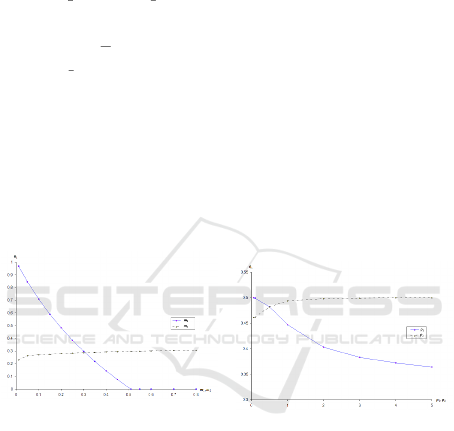
This requires numerical analysis. Figure 1 illus-
trates the effect of the retailer’s margin on the man-
ufacturer’s participation rate. We use the following
sample parameter values: r = 0.03, ρ
1
= ρ
2
= 0.5,
δ
1
= 0.07, δ
2
= 0.1, M
1
= 0.5, M
2
= 0.2. Further-
more, for the effect of Retailer 1’s margin, we set Re-
tailer 2’s margin to m
2
= 0.5, and vice versa.
We already know from Corollary 1(c) that
∂S/∂m < 0 at S ≤ 0 in the symmetric case. The result
shown in Figure 1—that θ
∗
1
decreases, and at a de-
ceasing rate, as the margin m
1
of the supported retailer
increases—is consistent with our finding in the sym-
metric case and represents its generalization to the
asymmetric case. The reason behind this result is that
Figure 1: Effect of Retailers’ Margins on the Optimal Par-
ticipation Rate.
with low margin m
1
, Retailer 1 will under-advertise
and the manufacturer’s profit will suffer. So, then, it
is in the interest of the manufacturer to participate so
as to encourage the retailer to advertise more. As m
1
increases, Retailer 1 has its own incentive to adver-
tise, and, therefore, the manufacturer does not need
to offer as much in the way of participation. As m
1
keeps increasing, the manufacturer ceases to partici-
pate altogether. We see from Figure 1 that θ
∗
1
indeed
becomes zero at m
1
≈0.5, where the switch from “co-
operative advertising” to “no cooperative advertising”
takes place. A more precise value can be obtained by
using (27), and we find this to be m
1
= 0.50925. Thus,
we have generalized to the competitive environment
the result obtained in He et al. (2009) in the absence
of competition.
The effect of the margin of the non-supported re-
tailer, i.e., Retailer 2, on the offer of cooperative
advertising to Retailer 1, the supported retailer, ap-
pears to be weak. Note that at m
1
= 0.3, the two
curves in Figure 1 cross. At this point, as m
1
in-
creases ceteris paribus, θ
∗
1
decreases sharply whereas
as m
2
increases, θ
∗
1
increases but slowly. This means
that as m
2
increases, Retailer 1 faces greater advertis-
ing competition from the competing retailer and this
induces the manufacturer to support Retailer 1 at a
slightly higher rate. On the other hand, as m
1
in-
creases, as has already been mentioned, it increases
the incentive of Retailer 1 to advertise of its own ac-
cord, and thus the manufacturer reduces its support
significantly. Even though m
2
has a weak effect on
θ
∗
1
, it may still make a difference between the manu-
facturer supporting or not supporting Retailer 1. Nu-
merical analysis shows that when m
1
= m
2
= 0.5,
then θ
∗
1
= 0.012. But as m
2
decreases from 0.5 (e.g.,
m
2
= 0.25), the manufacturer stops offering promo-
tional support to Retailer 1. On the other hand, as m
2
increases from 0.5 to 0.80, θ
∗
1
increases from a sup-
port of 1.2% to only 3.2%.
Figure 2: Effect of Advertising Effectiveness on the Opti-
mal Participation Rate.
In Figure 2, the fixed parameter values are m
1
=
0.2, m
2
= 0.5, r = 0.03, ρ
1
= 0.5, δ
1
= 0.07, δ
2
= 0.1,
M
1
= 0.5, M
2
= 0.2. Consistent with the comparative
statics result for the symmetric case in Corollary 1(c)
that ∂S/∂ρ < 0, this figure shows that as the advertis-
ing effectiveness of the supported retailer increases,
the degree of support by the manufacturer diminishes.
The reason is that, given the greater effectiveness of
advertising, the retailer has an incentive to advertise
at a higher level even without the support of the man-
ufacturer. The unsupported retailer’s advertising ef-
fectiveness does not have a great impact, but as it in-
creases, it slowly raises the participation rate.
Finally, Figure 3 shows that as the sum of the mar-
ket share decay rates for the two retailers increases,
Co-Op Advertising with Two Competing Retailers: A Feedback Stackelberg-Nash Game
25

Figure 3: Effect of Decay on the Optimal Participation Rate.
the participation rate to the supported retailer, i.e.,
Retailer 1, increases. For this figure, the remaining
parameter values are m
1
= 0.5, m
2
= 0.2, r = 0.03,
ρ
1
= 0.5, ρ
2
= 0.5, M
1
= 0.8, M
2
= 0.2. Note that
we have plotted θ
∗
1
against the sum of the decay rates
since it is clear from the dynamics in (1) that the de-
cay rate for Retailer 1 is (δ
1
+ δ
2
). It is for this rea-
son that we can easily see from equations (32-37) that
β
1
, β
2
, and β
M
, and, therefore, θ
∗
1
, are affected by the
sum (δ
1
+δ
2
) and not by the decay rates individually.
The result can be explained intuitively since the in-
crease of (δ
1
+ δ
2
) is similar to increasing the speed
of the treadmill with which the advertising must keep
up. Thus, as (δ
1
+ δ
2
) increases, Retailer 1 finds it
more expensive to maintain its market share and the
manufacturer must offer a higher participation rate to
Retailer 1 to adequately promote the product. This
finding generalizes to the asymmetric case the analyt-
ical result obtained for the symmetric case in Corol-
lary 1(c) that ∂S/∂δ < 0. Finally, note that the effect
of the decay rates is most pronounced at their lower
values and does not have much effect on the partici-
pation rate at higher values.
5 EXTENSIONS
The model can be extended to include retail price
competition. In the case where the retail price, de-
noted p
i
, is endogenously determined in addition to
the advertising decision u
i
, Retailer i’s discounted
profit maximization problem is given by
V
i
(x
0
) = max
u
i
(t), p
i
(t)
Z
∞
0
e
−rt
Ωdt i = 1, 2, (38)
subject to (1), where
Ω = D
i
(p
i
(t), p
3−i
(t))(p
i
(t) −c
i
)x
i
(t)
−(1 −θ
i
(x(t)))u
2
i
(t),
p
i
(t) is the price charged by Retailer i,
D
i
(p
i
(t), p
3−i
(t)) = (1 −b
i
p
i
(t) + d
3−i
p
3−i
(t))
is the demand function expressed as a function of the
prices of the two retailers, c
i
is the marginal cost of
Retailer i, and b
i
and d
i
are demand parameters. Solv-
ing for the retailers’ optimal prices yields
ˆp
i
=
d
3−i
+ b
3−i
(2 + 2b
i
c
i
+ d
3−i
c
3−i
)
4b
1
b
2
−d
1
d
2
, i = 1,2.
(39)
Using the parameter m
i
to denote
(D
i
(p
i
(t), p
3−i
(t)))(p
i
(t) −c
i
) in equation (38),
where p
i
= ˆp
i
from equation (39), results in equations
(2-3).
The demand parameters affect price, which, in
turn, affects the profit margins. Thus, the results in
Section 4 remain unchanged except that we can now
add that the demand parameters affect the participa-
tion rate θ
∗
1
via m
i
, i =1, 2.
As in Prasad and Sethi (2004), one could extend
the model to include a stochastic term in the dynamic
equation in (1) as follows:
dx (t) =
ρ
1
u
1
(t)
p
1 −x(t) −ρ
2
u
2
(t)
p
x (t)
dt
+(−δ
1
x (t) +δ
2
(1 −x(t)))dt
+σ(x(t))dz (t) (40)
where σ(x (t)) represents a variance term and z(t),
t ≥ 0, is the standard Wiener process.
6 CONCLUSIONS
In this paper, we consider a manufacturer who sells a
product to one or both of two independent and com-
peting retailers. The retailers invest in local adver-
tising effort, while the manufacturer decides whether
or not to support the retailers’ advertising activities
through a participation rate. We use differential game
theory to solve the Stackelberg game between the
manufacturer and the two retailers.
We derive the optimal advertising levels of the
two retailers and the participation rates of the man-
ufacturer, and find that the manufacturer will provide
strictly less than 100% participation rate, and that the
manufacturer will offer a non-zero participation rate
to the retailer from whom the manufacturer earns the
higher margin. We then analyzed several special cases
of the general model, including the case of symmetric
retailers. Compared to He et al. (2009), who do not
model retail competition, we find that the presence of
a competing retailer induces the manufacturer to pro-
vide a higher level of cooperative advertising support
ICORES 2020 - 9th International Conference on Operations Research and Enterprise Systems
26

to its retailer, and for a greater range of parameter val-
ues, than if that retailer were a monopolist.
There remain open issues for future research. To
preserve tractability, we did not model the manufac-
turer’s wholesale price decision in this paper, as was
done in He et al. (2009). Future research could extend
the model to also include the manufacturer’s whole-
sale price. It would also be interesting to explore deci-
sions in a retail oligopoly, along the lines of Fruchter
(1999).
Finally, this paper opens up a fruitful avenue for
future empirical research. Since we have provided
the optimal participation rates as well as their de-
pendence on various firm- and industry-level param-
eters, it would now be possible to empirically ex-
amine whether our results can explain the participa-
tion rates in different industries as reported in Dutta
et al. (1995). This would of course require estima-
tion of the firm- and industry-level parameters, pos-
sibly employing the techniques used in Naik et al.
(2008). Provided an appropriate data set can be found
or collected, an empirical study to validate our results
would undoubtedly deepen our understanding of the
cooperative advertising practices in different indus-
tries.
REFERENCES
F. M., A. Krishnamoorthy, A. Prasad, S. P. Sethi. 2005.
Generic and brand advertising strategies in a dynamic
duopoly. Marketing Science 24 556-568.
A., S. Chen, S. P. Sethi, 2014. Feedback Stackelberg
Solutions of Infinite-Horizon Stochastic Differential
Games. Models and Methods in Economics and Man-
agement Science, Essays in Honor of Charles S.
Tapiero, F.E. Ouardighi and K. Kogan (Eds.), Interna-
tional Series in Operations Research & Management
Science, Vol. 198, Springer 3-15.
A., S. Chen, S. P. Sethi, 2015. The Maximum Principle for
Global Solutions of Stochastic Stackelberg Differen-
tial Games. SIAM Journal on Control and Optimiza-
tion 53(4) 1956-1981.
A., S. Chen, S. P. Sethi, A. Chutani, C. C. Siu, S. C.
P. Yam. 2019 (forthcoming). Feedback Stackelberg–
Nash Equilibria In Mixed Leadership Games With an
application to cooperative advertising. SIAM Journal
on Control and Optimization.
M., G. John. 1997. Understanding cooperative advertising
participation rates in conventional channels. Journal
of Marketing Research 34 357-369.
P. D. 1972. Vertical cooperative advertising ventures. Jour-
nal of Marketing Research 9 309-312.
Berger P. D., T. Magliozzi. 1992. Optimal cooperative ad-
vertising decisions in direct-mail operations. Journal
of the Operational Research Society 43 1079-1086.
Chintagunta P. K., D. C. Jain. 1992. A dynamic model
of channel member strategies for marketing expendi-
tures. Marketing Science 11 168-188.
Dant R. P., P. D. Berger. 1996. Modeling cooperative adver-
tising decisions in franchising. Journal of the Opera-
tional Research Society 47 1120-1136.
Deal K. R. 1979. Optimizing advertising expenditures in a
dynamic duopoly. Operations Research 27 682-692.
Dockner E. J., S. Jørgensen, N. V. Long, and G. Sorger.
(2000). Differential Games in Economics and Man-
agement Science, Cambridge University Press, Cam-
bridge, UK.
Dutta S., M. Bergen, G. John, A. Rao. 1995. Variations in
the contractual terms of cooperative advertising con-
tracts: Am empirical investigation. Marketing Letters
6 15-22.
Erickson G. M. 2009. An oligopoly model of dynamic ad-
vertising competition. European Journal of Opera-
tional Research 197 374-388.
Fruchter G. E., 1999. The many-player advertising game.
Management Science 45 1609-1611.
He X., A. Krishnamoorthy, A. Prasad, S. P. Sethi. 2011.
Retail competition and cooperative advertising. Oper-
ations Research Letters 39 11-16.
He X., A. Krishnamoorthy, A. Prasad, S. P. Sethi. 2012. Co-
Op Advertising in Dynamic Retail Oligopolies. Deci-
sion Sciences Journal 43 73-105.
He X., A. Prasad, S. P. Sethi, G. Gutierrez. 2007. A sur-
vey of Stackelberg differential game models in supply
chain and marketing channels. Journal of Systems Sci-
ence and Systems Engineering 16 385-413.
He X., A. Prasad, S. P. Sethi. 2009. Cooperative advertis-
ing and pricing in a dynamic stochastic supply chain:
Feedback Stackelberg strategies. Production and Op-
erations Management 18 78-94.
Huang Z., S. X. Li. V. Mahajan. 2002. An analysis of
manufacturer-retailer supply chain coordination in co-
operative advertising. Decision Sciences 33 469-494.
Jørgensen S., S. P. Sigue, G. Zaccour. 2000. Dynamic coop-
erative advertising in a channel. Journal of Retailing
76 71-92.
Jørgensen S., S. Taboubi, G. Zaccour. 2001. Cooperative
advertising in a marketing channel. Journal of Opti-
mization Theory and Applications 110 145-158.
Jørgensen S., S. Taboubi, G. Zaccour. 2003. Retail promo-
tions with negative brand image effects: Is coopera-
tion possible? European Journal of Operational Re-
search 150 395-405.
Jørgensen S., G. Zaccour. 2003. Channel coordination over
time: Incentive equilibria and credibility. Journal of
Economic Dynamics and Control 27 801-822.
Karray S., G. Zaccour. 2005. A differential game of adver-
tising for national brand and store brands. In: A. Hau-
rie and G. Zaccour (Eds.), Dynamic Games: Theory
and Applications, Springer, 213-229.
Kim S. Y., R. Staelin. 1999. Manufacturer allowances and
retailer pass-through rates in a competitive environ-
ment. Marketing Science 18 59-76.
Nagler M. G. 2006. An exploratory analysis of the deter-
minants of cooperative advertising participation rates.
Marketing Letters 17 91-102.
Co-Op Advertising with Two Competing Retailers: A Feedback Stackelberg-Nash Game
27

Naik P. A., A. Prasad, S. P. Sethi. 2008. Building brand
awareness in dynamic oligopoly markets. Manage-
ment Science 54(1) 129-138.
Prasad A., S. P. Sethi. 2004. Competitive advertising under
uncertainty: A stochastic differential game approach.
Journal of Optimization Theory and Applications 123
163-185.
Sethi S. P. 1983. Deterministic and stochastic optimization
of a dynamic advertising model. Optimal Control Ap-
plications and Methods 4 179-184.
Sorger G. 1989. Competitive dynamic advertising: A mod-
ification of the Case game. Journal of Economic Dy-
namics and Control 13 55-80.
Vidale M. L., H. B. Wolfe. 1957. An operations-research
study of sales response to advertising. Operations Re-
search 5 370-381.
APPENDIX
Proof of Proposition 1
First, note that if M
1
> M
2
, then the
manufacturer’s objective function in equa-
tion (4) can be organized as follows:
R
∞
0
e
−rt
M
2
+ (M
1
−M
2
)x −θ
1
u
2
1
(x) −θ
2
u
2
2
(x)
dt.
This suggests that the manufacturer should encourage
Retailer 1 to increase its advertising to increase x
(and discourage Retailer 2 to decrease advertising
and (1 −x) by setting θ
∗
2
= 0) as much as possible.
xspace
Proof of Proposition 2
The Hamilton-Jacobi-Bellman (HJB) equation (Sethi
and Thompson 2000) for Retailer i is given by:
rV
1
= max
u
1
n
m
1
x −(1 −θ
1
)u
2
1
+V
0
1
ρ
1
u
1
√
1 −x
−V
0
1
ρ
2
u
2
√
x −δ
1
x + δ
2
(1 −x)
o
, (41)
rV
2
= max
u
2
m
2
(1 −x) −(1 −θ
2
)u
2
2
+V
0
2
ρ
1
u
1
√
1 −x
−V
0
2
ρ
2
u
2
√
x −δ
1
x + δ
2
(1 −x)
o
.(42)
The first-order conditions for maximization yield the
optimal advertising levels in equation (8) in Proposi-
tion 2(a). Substituting these solutions into the above
HJB equations for the two retailers yields equations
(10-11) in Proposition 2(c).
The HJB equation for the manufacturer is given
by:
rV = max
θ
1
, θ
2
M
1
x + M
2
(1 −x) −θ
1
u
2
1
(x|θ
1
,θ
2
)
−θ
2
u
2
2
(x|θ
1
,θ
2
)
+V
0
ρ
1
u
1
(x|θ
1
,θ
2
)
√
1 −x
−V
0
(ρ
2
u
2
(x|θ
1
,θ
2
)
√
x −δ
1
x + δ
2
(1 −x)).
(43)
Substituting the optimal advertising efforts of the
two retailers into the above equation and simplifying
yields
rV = max
θ
1
, θ
2
M
1
x + M
2
(1 −x) −
1
4
θ
1
ρ
2
1
V
0
1
2
(1−x)
(1−θ
1
)
2
+
θ
2
ρ
2
2
V
0
2
2
x
(1−θ
2
)
2
!
−
(1−θ
1
)ρ
2
2
V
0
2
x+(1−θ
2
)
2(δ
1
x−δ
2
(1−x))(1−θ
1
)−ρ
2
1
V
0
1
(1−x)
2(1−θ
1
)(1−θ
2
)
!
V
0
.
(44)
Solving the first-order conditions for the partici-
pation rates, and noting that M
1
> M
2
implies θ
∗
2
= 0,
yields equation (9) in Proposition 2(b). Substituting
these solutions into equation (44) and simplifying, we
obtain equation (12) in Proposition 2(c). xspace
Proof of Proposition 3
With V
1
= α
1
+β
1
x and V
2
= α
2
+β
2
(1 −x), we have
V
0
1
= β
1
and V
0
2
= β
2
. Inserting these into (10) and
(11), we have
r (α
1
+ β
1
x) = m
1
x +
β
2
1
ρ
2
1
(1 −x)
4
1 −
2V
0
−β
1
2V
0
+β
1
+
−
β
1
β
2
ρ
2
2
x
2
−β
1
(δ
1
x −δ
2
(1 −x)), (45)
r (α
2
+ β
2
(1 −x)) = m
2
(1 −x) +
β
2
2
ρ
2
2
x
4
−
β
1
β
2
ρ
2
1
(1 −x)
2
1 −
2V
0
−β
1
2V
0
+β
1
+
+ β
2
(δ
1
x −δ
2
(1 −x)). (46)
With V = α
M
+ β
M
x, we have V
0
= β
M
. Substi-
tution into equations (8) and (9) yields (13) in Propo-
sition 3(a) and (14) in Proposition 3(b), respectively.
Substituting these into the HJB equation in (12) and
simplifying yields
r (α
M
+ β
M
x) = M
1
x + M
2
(1 −x) −
β
2
β
M
ρ
2
2
x
2
−
β
2
1
ρ
2
1
2β
M
−β
1
2β
M
+β
1
+
(1 −x)
4
1 −
2β
M
−β
1
2β
M
+β
1
+
2
−
β
1
β
M
ρ
2
1
(1 −x)
2
1 −
2β
M
−β
1
2β
M
+β
1
+
−δ
1
β
M
x + δ
2
β
M
(1 −x). (47)
ICORES 2020 - 9th International Conference on Operations Research and Enterprise Systems
28

Equating the powers of x in (47), we obtain equa-
tions (19-20) in Proposition 3(c). Substituting V
0
=
β
M
into (45-46) and equating the powers of x and
(1 −x) yields equations (15-18) in Proposition 3(c).
xspace
Proof of Proposition 4
Solving equation (22) for β
2
yields
β
2
=
4m
1
−β
1
β
1
ρ
2
1
+ 4(r + δ
1
+ δ
2
)
2β
1
ρ
2
2
. (48)
Substituting the above solution into equation (24) and
simplifying yields the quartic equation (28).
As detailed in Prasad and Sethi (2004), it can be
shown that there exists a unique β
1
> 0 that solves the
above quartic equation. This is the unique equilibrium
of the Stackelberg differential game. That solution
can then be substituted into (48) to yield the solution
for β
2
. We know from (26) that
β
M
=
2(M
1
−M
2
)
β
1
ρ
2
1
+ β
2
ρ
2
2
+ 2(r + δ
1
+ δ
2
)
. (49)
Substituting the solutions for β
1
and β
2
into (49)
yields β
M
.
Since β
M
> 0 from equation (20), the participation
threshold is obtained as 2β
M
−β
1
as follows;
4(M
1
−M
2
) −β
2
1
ρ
2
1
−β
1
β
2
ρ
2
2
−2β
1
(r + δ
1
+ δ
2
)
β
1
ρ
2
1
+ β
2
ρ
2
2
+ 2 (r + δ
1
+ δ
2
)
. (50)
We know from equation (22) that
β
1
β
2
ρ
2
2
+ 2β
1
(δ
1
+ δ
2
) =
1
2
4m
1
−4rβ
1
−β
2
1
ρ
2
1
.
Using this in the numerator of (50) and simplify-
ing gives the participation threshold S in (27).
Since β
1
is independent of (M
1
−M
2
), we have
∂S/∂(M
1
−M
2
) = 2 > 0. xspace
Proof of Corollary 1
The solutions for α
i
and β
i
, i = 1,2, in Corollary 1(a),
are the same as in the symmetric analysis in Prasad
and Sethi (2004) in the absence of uncertainty.
For the manufacturer, as before, the linear value
function V = α
M
+β
M
x solves the HJB equation. Set-
ting θ
1
= θ
2
= 0, imposing symmetry in the model
parameters, and simplifying the HJB equation results
in
r(α
M
+ β
M
x) = M
2
+
β
M
βρ
2
+ 2δ
2
+
M
1
−M
2
−
βρ
2
+ 4δ
2
β
M
x. (51)
Equating the coefficients of x in equation (51)
yields the solutions in equation (30) in Corol-
lary 1(b). Note that this can be interpreted as
R
∞
0
e
−rt
(M
1
x + M
2
(1 −x))dt given the solution ob-
tained with θ
1
= θ
2
= 0.
For the comparative statics, imposing symmetry
in the participation threshold from equation (27), we
have S(.) = 2(M
1
−M
2
) −m −
β
2
ρ
2
4
= 0. Substitut-
ing the solution for β from equation (29), this can be
rewritten as
S(.) = 2(M
1
−M
2
) −
4
3
m
+
2(r + 2δ)
p
(r + 2δ)
2
+ 3mρ
2
−(r + 2δ)
9ρ
2
. (52)
Taking the derivative of S in equation (52) w.r.t.
the model parameters yields the comparative statics
in Corollary 1(c): ∂S/∂(M
1
−M
2
) > 0, ∂S/∂m < 0,
∂S/∂ρ < 0, ∂S/∂r > 0, ∂S/∂δ > 0.
Proof of Corollary 2
We know that V
0
= β
M
and β
1
= β
2
= β, where
β =
√
(r+2δ)
2
+3mρ
2
−(r+2δ)
3ρ
2
/2
. Moreover, β
M
=
M
1
−M
2
βρ
2
+r+2δ
,
with the aforementioned β.
Since θ
1
=
2V
0
−β
1
2V
0
+β
1
=
2β
M
−β
2β
M
+β
, we need 2β
M
−β > 0
for θ
1
> 0. Substituting the value of β into β
M
and
simplifying 2β
M
−β, we have
S = 2β
M
−β =
6(M
1
−M
2
)
r + 2δ + 2
p
(r + 2δ)
2
+ 3mρ
2
−
2
q
3mρ
2
+ (r + 2δ)
2
−(r + 2δ)
3ρ
2
. (53)
Therefore, θ
∗
1
> 0 when S > 0 from above. With
r = δ = 0 in (53), we obtain equation (31) as the ap-
proximation of (53). xspace
Co-Op Advertising with Two Competing Retailers: A Feedback Stackelberg-Nash Game
29
