Detection of Lattice-points inside Triangular Mesh for Variable-viscosity
Model of Red Blood Cells
Tibor Po
ˇ
stek, Franti
ˇ
sek Kaj
´
anek and Mariana Ondru
ˇ
sov
´
a
Cell-in-Fluid Biomedical Modelling and Computations Group, Faculty of Management Science and Informatics,
University of
ˇ
Zilina, Slovakia
Keywords:
Deformable Objects, Lattice-Boltzmann Method, Variable Fluid Viscosity.
Abstract:
In this work we introduce the extension of an existing computational model for red blood cells that enables
modelling of different viscosity inside and outside the cells. The extension is based on an algorithm for
detection of fluid lattice-points inside the cell given the membrane of the cell as a closed triangular mesh. This
algorithm enables the setting of variable viscosity in the underlying lattice-Boltzmann method for computation
of fluid dynamics.
1 INTRODUCTION
Computational models serve a wide variety of roles,
including hypothesis testing, generating new insights,
deepening understanding, suggesting and interpreting
experiments, tracing chains of causation or perform-
ing sensitivity analyses. Computational modelling
helps to predict outcomes in circumstances that are
difficult to achieve in laboratory (Calder and et al.,
2018). Model cannot replace experiment, but it can
demonstrate whether or not a proposed mechanism
is sufficient to produce an observed phenomenon.
Model can be an effective tool in optimization and
design (Janacek et al., 2017; Kleineberg et al., 2017).
Computational modelling helps to predict out-
comes in circumstances that are difficult to achieve in
laboratory (Calder and et al., 2018). It is an effective
tool in optimization and design (Janacek et al., 2017;
Kleineberg et al., 2017).
Computational modelling of deformable objects
immersed in a flow such as biological cells inside
microfluidic devices (Bu
ˇ
s
´
ık et al., 2016; Gusenbauer
et al., 2018; Jan
ˇ
cigov
´
a and Cimr
´
ak, 2016; Cimrak,
2016; Reichel et al., 2019), requires capturing various
bio-mechanical phenomena. One such example is dif-
ferent fluid viscosities inside and outside the cell. For
example, red blood cells (RBC) are composed of cell
membrane and the inner fluid called cytoplasm. Cy-
toplasm has four to five times higher viscosity than
plasma surrounding red blood cells. Similar scenario
holds for other cells or other environments, for exam-
ple when various kinds of cells are manipulating in
microfluidic devices.
Several computational models of RBC do not con-
sider the difference between inner and outer fluid vis-
cosities (Krueger, 2012; Dupin et al., 2007; Schiller
et al., 2018) while others include this possibility
(Doddi and Bagchi, 2009; Fedosov et al., 2010).
There is an ongoing discussion about the necessity
to consider variable viscosity, although it has been
shown in (Fedosov et al., 2010), that different inner
viscosity lead to different rotational behaviour of red
blood cells in a shear flow.
The principal algorithmic task that is needed to be
solved is to determine all spatial points in a three-
dimensional space that lie within closed surface. In
particular, we are interested only in those points with
coordinates being integer numbers that are enclosed
by a triangulation of a closed surface. The triangu-
lation mesh-points can have non-integer coordinates.
This specification comes from the fact that the fluid is
discretized by a fixed lattice - therefore fluid nodes
have integer coordinates, and the cell membrane is
discretized by a triangular network.
This algorithmic task seems to be similar to
task solved e.g. in Computational Geometry Algo-
rithms Library project in a highly optimized manner.
CGAL’s particular package (Loriot et al., 2019) has
been designed to handle huge triangular meshes and
to manipulate them, for example find intersections of
two meshes, or, decide whether a point in 3D space is
inside or outside the mesh.
Our case is however different: We need to make
such decision for all lattice points in space. There-
212
Poštek, T., Kajánek, F. and Ondrušová, M.
Detection of Lattice-points inside Triangular Mesh for Variable-viscosity Model of Red Blood Cells.
DOI: 10.5220/0009165102120217
In Proceedings of the 13th International Joint Conference on Biomedical Engineering Systems and Technologies (BIOSTEC 2020) - Volume 3: BIOINFORMATICS, pages 212-217
ISBN: 978-989-758-398-8; ISSN: 2184-4305
Copyright
c
 2022 by SCITEPRESS – Science and Technology Publications, Lda. All rights reserved

fore, the use of CGAL is quite limited because run-
ning over all lattice points we get cubic computational
complexity. We further discuss the topic of complex-
ity in Section 4.2.
In this work we provide a basic study of an ex-
tension of existing RBC model to include the pos-
sibility of various viscosities inside and outside the
cell. In Section 2, we provide description of un-
derlying model for the fluid and the notion of non-
constant viscosity. Next in Section 3 we analyze in
detail how non-constant viscosity is implemented in
the lattice-Boltzmann model of fluid flow. In Section
4 we present our algorithm, with discussion on com-
plexity.
2 NON-CONSTANT VISCOSITY
IN MODELLING OF
DEFORMABLE OBJECTS
We have been using the lattice-Boltzmann method
(LBM) coupled with the spring network method for
modelling of flow of deformable objects in a fluid
(Cimr
´
ak et al., 2012; Cimr
´
ak et al., 2014). Here,
the LBM governs the evolution of the fluid while the
spring network is used to characterize the boundary
of the immersed object. The LBM and the spring net-
work is coupled by a dissipative coupling penalizing
the difference between the velocities of the fluid and
the spring network mesh points.
This method has been previously used for simula-
tions of blood cells, having uniform fluid viscosity in-
side and outside the cell. In reality however, the inner
fluid of red blood cells has four times higher viscosity
than the surrounding fluid. Original implementation
presented in (Cimr
´
ak et al., 2012; Cimr
´
ak et al., 2014)
concerns the case of constant fluid viscosity.
We aim at introducing the possibility to account
for variable viscosity. Therefore we will consider
a spatial and time dependent kinematic viscosity
ν
s
(~x,t) instead of the constant kinematic viscosity.
From now on, if we mention viscosity, we mean kine-
matic viscosity of the fluid. Bearing in mind our field
of application being the modelling of blood or tumour
cells, we will consider ν
s
(~x,t) to be a multi valued
piece-wise constant function for each time instance
t. Since multiple cell types could be involved, we will
work with possibility to have several different viscosi-
ties of the inner fluid of the cells, depending on the
type of cells. For example, red blood cells have dif-
ferent viscosity of cytoplasm than white blood cells.
Definition of variable viscosity function will be
ν
s
(~r,t) =

ν
i
, if~r lies inside a cell of type i
ν
0
, if~r lies outside any cells
(1)
where ν
i
is the shear viscosity of the inner fluid of
the cells of type i, and ν
0
is the shear viscosity of the
outer fluid.
To justify the possibility to use variable fluid vis-
cosity in LBM, we present several such cases when
lattice-Boltzmann method has been used also for
cases of non-constant fluid viscosity. Viscosity of the
fluid may change for example with temperature, shear
or concentration. Laminar convection of a fluid with a
temperature-dependent viscosity in an enclosure filled
with a porous medium was studied in (Guo and Zhao,
2005). The authors used lattice-Boltzmann method
combined with heat transfer equation.
In (Wang and Ho, 2011) the authors use new
lattice Boltzmann approach within the framework
of D2Q9 lattice for simulating shear-thinning non-
Newtonian blood flows described by the power-law.
In (Chao et al., 2007) the authors consider variable
viscosity complicating the truncation error analysis
and creating additional interaction between the trun-
cation error and the boundary condition error. In
(Rakotomalala et al., 1996) the authors address the
use of LBM for flows in which the viscosity is space
and time dependent, namely for non-Newtonian flu-
ids with shear dependent viscosity and miscible fluids
with concentration dependent viscosity.
The case of multiple-relaxation-time lattice-
Boltzmann method for incompressible miscible flow
with large viscosity ratio and high P
´
eclet number
was studied in (Meng and Guo, 2015). Authors in
(Krafczyk and Toelke, 2003) include Smagorinsky’s
algebraic eddy viscosity approach into the multiple-
relaxation- time lattice Boltzmann equation for large-
eddy simulations of turbulent flows. The inclusion
of variable viscosity is enabled by three-dimensional
multi-relaxation time lattice-Boltzmann models for
multi-phase flow presented in (Premnath and Abra-
ham, 2007).
3 LATTICE-BOLTZMANN
METHOD IN THE
COMPUTATIONAL MODEL
After we justified the possibility to use variable vis-
cosity in the LBM we looked closely on how to im-
plement the variable viscosity into the LBM. We work
with LBM described in (Dunweg and Ladd, 2009;
Weik et al., 2019). This model has been implemented
Detection of Lattice-points inside Triangular Mesh for Variable-viscosity Model of Red Blood Cells
213

in ESPResSo (Arnold et al., 2013) which is a scien-
tific package that we have been using. In ESPResSo, a
three-dimensional lattice-Boltzmann model is imple-
mented where velocity space is discretized in 19 ve-
locities (D3Q19 model). The details about this model
are available in (Dunweg and Ladd, 2009). The col-
lision step is performed after a transformation of the
populations into mode space. This allows implemen-
tation of the multiple relaxation time (MRT) lattice-
Boltzmann method (Lallemand et al., 2003). It also
allows the use different relaxation times for different
modes, thus to adjust the bulk and shear viscosity of
the fluid separately.
Bulk vs Shear Viscosity. Common notion of
viscosity refers mostly to shear viscosity. Shear vis-
cosity is the resistance of the fluid against shearing
motion. It is present e.g. in the Couette flow: Two
parallel plates are moving in the opposite directions
generating shear flow. The layers of liquid in dif-
ferent heights are moving with different velocities,
the friction between them arises that generate the re-
sistance against such movement. This resistance is
called shear viscosity.
Bulk viscosity refers to resistance of the fluid
against shear-less compression or expansion of the
fluid. For incompressible liquids the bulk viscosity
does not enter the hydrodynamic equations at all.
Mode Space. The principle of the mode space
is that populations are transformed into modes. There
are 19 modes, denoted by indexes 0 to 18. Modes 0-
3 correspond to the conserved variables, mass density
ρ, and momentum density j. Moments 4-9 correspond
to bulk and shear stresses. These moments also affect
the viscosity of the fluid. The higher modes 10-18
represent kinetic modes, they do not enter bulk hydro-
dynamic equations, but they play a role near bound-
aries and in thermal fluctuations.
For the implementation of relaxation time, there
are two possibilities in ESPResSo: The multiple-
relaxation-time or two-relaxation-time (TRT). The
TRT model is described in (Chun and Ladd, 2007).
These two possibilities have two different sets of
eigenvectors and eigenvalues of the collision operator.
They are shown in Table 1 in (Chun and Ladd, 2007).
We will consider the MRT case. Here, the eigenvalues
for the first four modes are zero, for mode 4 we have
eigenvalue γ
b
corresponding to dynamic bulk viscos-
ity µ
b
and for modes 5-9 we have eigenvalue γ
s
cor-
responding to dynamic shear viscosity µ
s
. Exact rela-
tion between eigenvalues and viscosities are given by
Equation 80 and 81 from (Dunweg et al., 2007)
µ
s
=
τρc
2
s
2
1 + γ
s
1 −γ
s
µ
b
=
τρc
2
s
d
1 + γ
b
1 −γ
b
Here, ρ is the fluid density, τ is the time step and c
s
is
the speed of sound in the LB lattice, namely
c
s
=
1
√
3
b
τ
where b is the lattice spacing. So when the γ
s
needs to
be evaluated for given viscosity, we plug expression
for c
s
to get
µ
s
=
τρ
2
b
2
3τ
2
1 + γ
s
1 −γ
s
=
ρb
2
6τ
1 + γ
s
1 −γ
s
1 + γ
s
1 −γ
s
=
6τµ
s
ρb
2
If kinematic viscosity ν
s
= µ
s
/ρ is used, the fluid den-
sity ρ vanishes from the expressions
1 + γ
s
1 −γ
s
=
6τν
s
b
2
After some computations, one gets
γ
s
=
6τν
s
b
2
−1
6τν
s
b
2
+ 1
= 1 −
2
6τν
s
b
2
+ 1
which is exactly the relation implemented in a lb.cpp
file of the lb_reinit_parameters() function in
the ESPResSo core code.
Eventually, we have localized the relation that tells
us dependence of γ
s
and ν
s
and at this place in the
code we need to set different viscosities for the inner
fluid of the cells and outer fluid.
4 ALGORITHMS FOR
DETECTION OF CELL INNER
SPACE
Practical question is how to determine whether you
are inside or outside the cell. The fluid in LBM is
discretized by a fixed perpendicular 3D grid. For ease
of explanation, assume this grid has spacing 1. The
cell on the other hand is discretized by a triangular
mesh that covers its surface. This mesh is not linked
to the grid, it can freely deform according to the
mechanics of the membrane. So the problem can be
stated in the following way:
Find all points in 3D with coordinates being
natural numbers that are enclosed inside a given
triangular network.
We have developed efficient algorithms that solve
BIOINFORMATICS 2020 - 11th International Conference on Bioinformatics Models, Methods and Algorithms
214

this problem and we have described them in detail
in (Po
ˇ
stek, 2019). The basic idea of the algorithm
is to loop over all horizontal lines parallel to x axis
direction with coordinates being natural numbers.
For each such line, we note an ”entering” mark
whenever we detect crossing with any triangle from
the cell’s mesh, meaning we are coming from the
outside into the inside of the cell. When the second
such mark occurs, this means we are leaving the cell
and we mark it as ”exiting” mark.
After such loop we just loop again over horizon-
tal lines and all the grid points that lie between two
”entering” and ”exiting” marks are flagged to be in-
side the cell. All other grid points are automatically
outside the cell.
4.1 Algorithm Details
To find an intersection of all lines along x axis direc-
tion with remaining two coordinates natural numbers,
we do it in an loop over y-coordinate. For a fixed y-
coordinate we need to find all intersections of mesh
triangles with plane with the same y-coordinate and
parallel to x and z axis, we denote this plane as Y-
plane. In Figure 1 you can see the visualization of
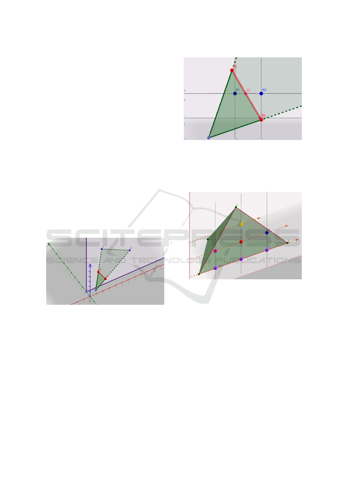
such intersection.
Figure 1: Points P
1
and P
2
characterize the intersection of a
triangle with Y-plane.
After identification of segment P
1
P
2
that is the in-
tersection of a triangle ABC (one of the mesh trian-
gles) with Y-plane, we need to detect the intersec-
tions of all horizontal lines from Y-plane that have
z-coordinate a natural number, see Figure 2
After obtaining the ”entering” and ”exiting”
marks on each horizontal line with natural y and z
coordinates, the loop over all lines will flag the in-
dividual grid points as inner or outer grid points, see
Figure 3.
Figure 2: Segment P
1
P
2
is the intersection of triangle with
plane y = integer number. Points Z
1
,Z
2
are those with inte-
ger z−coordinate and those are the intersections of horizon-
tal lines with segment P
1
and P
2
. Points X
1
,X
2
are the points
on horizontal lines that have integer x−coordinate. These
points are either ”entering” or ”exiting” mark for given hor-
izontal line, depending on the orientation of triangle ABC.
Figure 3: Variants of marking inside LB nodes.
4.2 Computational Efficiency
Consider a cubic computational domain with its edge
divided into n points. This leads to n
3
fluid lattice
points. In case of a single object (one cell in a simula-
tion), we need to decide about all n
3
points, whether
they are inside or outside the object described by a
mesh with N triangles. In our algorithm, we first
run over N triangles, and we create a list of enter-
ing and exiting marks for each horizontal line. Since
the number of horizontal lines in n
2
, this gives us
O(N ×n
2
) operations. Afterwards, we run over all lat-
tice points with O(n
3
) complexity, and we mark them
as inside or outside points according to entering and
exiting marks: If they lie between entering and exiting
mark, we mark them inside lattice points, otherwise
we mark them as outside lattice points. Both opera-
tions result in combined O(N ×n
2
)+ O(n
3
) complex-
ity.
Detection of Lattice-points inside Triangular Mesh for Variable-viscosity Model of Red Blood Cells
215

To compare our algorithm to the established
CGAL computational library: In CGAL, there is an
available package Polygon Mesh Processing and its
class CGAL::Side of triangle mesh that can decide
for a given point in space whether it lies inside or out-
side the triangular mesh. In order to mark all lattice
points as inside or outside points, we need to run the
functor of the class CGAL::Side of triangle mesh n
3
times. The complexity of the class is O(N), since it
needs to run over all triangles. Therefore, combined
complexity of CGAL algorithm is O(n
3
×N).
To wrap up, our algorithm with O(n
3
+ N × n
2
)
complexity is more efficient than CGAL algorithm
with O(N ×n
3
) complexity.
Speed-up
The presented algorithm has complexity O(n
3
+ N ×
n
2
), assuming the computational domain is a cube
with n discretization points on its edge. This might
still be too demanding for computations and if this
algorithm is executed in each time step, the computa-
tions will be dramatically slowed down.
To spare time, we propose to run this algorithm
in the beginning of the simulation to detect the cells’
interiors. Afterwards, once in a hundred time steps,
the algorithm can be executed again. Meanwhile, in
each time step a more sophisticated update algorithm
will be executed. The update algorithm will not run
over all horizontal lines and over all mesh points on
the lines, but it will only reflag the nearest grid points
near the mesh triangles. The update algorithm will
loop over all triangles in the mesh - which makes it
O(n
2
×N) complex - and after detecting the points in
the triangle with y and z coordinates natural numbers,
one can reflag the neighbouring grid points with all
coordinates natural numbers. This update algorithm
will be useful only in scenarios when during one time
step, the triangles from the mesh do not jump over
more than one grid point from the fluid discretization.
But in most simulations, the cell deforms and moves
slow enough so that it does not skip several fluid grid
points in one time step.
5 CONCLUSIONS AND
OUTLOOK
The presented algorithm enables the use of various
viscosity in an existing implementation of blood cell
modelling in ESPResSo. There must be several steps
done before claiming this algorithm is correct and ef-
ficient and before it can be used by the scientific com-
munity:
• Computational analysis of computational costs of
the algorithm. One must be sure that the intro-
duction of this algorithm to LBM method will not
slow the computations down rapidly.
• The whole implementation must be tested against
experimental and analytical data. The work
of (Feng and Michaelides, 2001) for example
includes tables of drag coefficients of viscous
spheres in a uniform flow. This could be simulated
and the computational drag coefficient compared
to those from (Feng and Michaelides, 2001).
ACKNOWLEDGEMENTS
This work was supported by the Slovak Research
and Development Agency (contract number APVV-
15-0751) and by the Ministry of Education, Science,
Research and Sport of the Slovak Republic (contract
number VEGA 1/0643/17).
REFERENCES
Arnold, A., Lenz, O., Kesselheim, S., Weeber, R., Fahren-
berger, F., Roehm, D., Ko
ˇ
sovan, P., and Holm, C.
(2013). ESPResSo 3.1 - molecular dynamics soft-
ware for coarse–grained models. In Griebel, M. and
Schweitzer, M., editors, Meshfree Methods for Partial
Differential Equations VI, Lecture Notes in Compu-
tational Science and Engineering, volume 89, pages
1–23.
Bu
ˇ
s
´
ık, M., Jan
ˇ
cigov
´
a, I., T
´
othov
´
a, R., and Cimr
´
ak, I.
(2016). Simulation study of rare cell trajectories and
capture rate in periodic obstacle arrays. Journal of
Computational Science, 17(2):370–376.
Calder, M. and et al. (2018). Computational modelling for
decision-making: where, why, what, who and how. R
Soc Open Sci, 5(6).
Chao, J., Mei, R., and Shyy, W. (2007). Error assessment of
lattice boltzmann equation method for variable viscos-
ity flows. International journal for numerical methods
in fluids, 53:1457–1471.
Chun, B. and Ladd, A. (2007). Interpolated boundary con-
dition for lattice boltzmann simulations of flows in
narrow gaps. Physical Review E, 75:066705.
Cimrak, I. (2016). Collision rates for rare cell capture in
periodic obstacle arrays strongly depend on density of
cell suspension. Computer Methods in Biomechanics
and Biomedical Engineering, 19(14):1525–1530.
Cimr
´
ak, I., Gusenbauer, M., and Jan
ˇ
cigov
´
a, I. (2014).
An ESPResSo implementation of elastic objects im-
mersed in a fluid. Computer Physics Communications,
185(3):900–907.
Cimr
´
ak, I., Gusenbauer, M., and Schrefl, T. (2012). Mod-
elling and simulation of processes in microfluidic de-
BIOINFORMATICS 2020 - 11th International Conference on Bioinformatics Models, Methods and Algorithms
216

vices for biomedical applications. Computers and
Mathematics with Applications, 64(3):278–288.
Doddi, S. and Bagchi, P. (2009). Three-dimensional compu-
tational modeling of multiple deformable cells flow-
ing in microvessels. Phys. Rev. E, 79(4):046318.
Dunweg, B. and Ladd, A. J. C. (2009). Lattice-Boltzmann
simulations of soft matter systems. Advances in Poly-
mer Science, 221:89–166.
Dunweg, B., Schiller, U., and Ladd, A. J. C. (2007). Sta-
tistical mechanics of the fluctuating lattice boltzmann
equation. Physical Review E??, 76:036704.
Dupin, M. M., Halliday, I., Care, C. M., and Alboul, L.
(2007). Modeling the flow of dense suspensions of de-
formable particles in three dimensions. Physical Re-
view E, Statistical, nonlinear, and soft matter physics,
75:066707.
Fedosov, D. A., Caswell, B., and Karniadakis, G. E. (2010).
A multiscale red blood cell model with accurate me-
chanics, rheology and dynamics. Biophysical Journal,
98(10):2215–2225.
Feng, Z. G. and Michaelides, E. E. (2001). Drag coefficients
of viscous spheres at intermediate and high reynolds
numbers. Journal of Fluids Engineering, 123:841–
849.
Guo, Z. and Zhao, T. (2005). Lattice boltzmann simulation
of natural convection with temperature-dependent vis-
cosity in a porous cavity. Progress in Computational
Fluid Dynamics, 5(1):110–117.
Gusenbauer, M., T
´
othov
´
a, R., Mazza, G., Brandl, M.,
Schrefl, T., Jan
ˇ
cigov
´
a, I., and Cimr
´
ak, I. (2018).
Cell damage index as computational indicator for
blood cell activation and damage. Artificial Organs,
42(7):746–755.
Janacek, J., Kohani, M., Koniorczyk, M., and Marton, P.
(2017). Optimization of periodic crew schedules with
application of column generation method. Trans-
portation Research Part C: Emerging Technologies,
83:165 – 178.
Jan
ˇ
cigov
´
a, I. and Cimr
´
ak, I. (2016). Non-uniform force al-
location for area preservation in spring network mod-
els. International Journal for Numerical Methods in
Biomedical Engineering, 32(10):e02757–n/a.
Kleineberg, K.-K., Buzna, L., Papadopoulos, F., Bogu
˜
n
´
a,
M., and Serrano, M. A. (2017). Geometric correla-
tions mitigate the extreme vulnerability of multiplex
networks against targeted attacks. Phys. Rev. Lett.,
118:218301.
Krafczyk, M. and Toelke, J. (2003). Large-edd simulations
with multiple-relaxation time lbe model. International
Journal of Modern Physics B, 17(1):33–39.
Krueger, T. (2012). Computer Simulation Study of Collec-
tive Phenomena in Dense Suspensions of Red Blood
Cells under Shear. PhD thesis, Max-Planck Institut.
Lallemand, P., d’Humieres, D., Luo, L., and Rubinstein,
R. (2003). Theory of the lattice boltzmann method:
three-dimensional model for linear viscoelastic fluids.
Phys. Rev. E, 67:021203.
Loriot, S., Rouxel-Labb
´
e, M., Tournois, J., and Yaz, I. O.
(2019). Polygon mesh processing. In CGAL User
and Reference Manual. CGAL Editorial Board, 5.0
edition.
Meng, X. and Guo, Z. (2015). Multiple-relaxation-time
lattice boltzmann model for incompressible miscible
flow with large viscosity ratio and high p
´
eclet num-
ber. PHYSICAL REVIEW E, 92:043305.
Po
ˇ
stek, T. (2019). Fluid dynamics model of cells with vari-
able inner and outer fluid viscosity. In Mathematics in
science and technologies [print] : proceedings of the
MIST conference 2019, pages 65–72.
Premnath, K. and Abraham, J. (2007). Three-dimensional
multi-relaxation time (mrt) lattice-boltzmann mod-
els for multiphase flow. Journal of Computational
Physics, 224:539–559.
Rakotomalala, N., Salin, D., and Watzky, P. (1996). Simu-
lations of viscous flows of complex fluids with a bhat-
nagar, gross, and krook lattice gas. Physics of Fluids,
8:3200–3202.
Reichel, F., Mauer, J., Nawaz, A. A., Gompper, G., Guck,
J., and Fedosov, D. A. (2019). High-throughput
microfluidic characterization of erythrocyte shapes
and mechanical variability. Biophysical Journal,
117(1):14 – 24.
Schiller, U. D., Kr
¨
uger, T., and Henrich, O. (2018). Meso-
scopic modelling and simulation of soft matter. Soft
Matter, 14:9–26.
Wang, C. and Ho, J. (2011). A lattice boltzmann approach
for the non-newtonian effect in the blood flow. Com-
puters and Mathematics with Applications, 62:75–86.
Weik, F., Weeber, R., Szuttor, K., Breitsprecher, K.,
de Graaf, J., Kuron, M., Landsgesell, J., Menke, H.,
Sean, D., and Holm, C. (2019). Espresso 4.0 – an
extensible software package for simulating soft mat-
ter systems. The European Physical Journal Special
Topics, 227(14):1789–1816.
Detection of Lattice-points inside Triangular Mesh for Variable-viscosity Model of Red Blood Cells
217