
Automatic Estimation of Sphere Centers from Images of Calibrated
Cameras
Levente Hajder, Tekla T
´
oth and Zolt
´
an Pusztai
Department of Algorithms and Their Applications, E
¨
otv
¨
os Lor
´
and University,
P
´
azm
´
any P
´
eter stny. 1/C, H-1117, Budapest, Hungary
Keywords:
Ellipse Detection, Spatial Estimation, Calibrated Camera, 3D Computer Vision.
Abstract:
Calibration of devices with different modalities is a key problem in robotic vision. Regular spatial objects,
such as planes, are frequently used for this task. This paper deals with the automatic detection of ellipses in
camera images, as well as to estimate the 3D position of the spheres corresponding to the detected 2D ellipses.
We propose two novel methods to (i) detect an ellipse in camera images and (ii) estimate the spatial location of
the corresponding sphere if its size is known. The algorithms are tested both quantitatively and qualitatively.
They are applied for calibrating the sensor system of autonomous cars equipped with digital cameras, depth
sensors and LiDAR devices.
1 INTRODUCTION
Ellipse fitting in images has been a long researched
problem in computer vision for many decades (Prof-
fitt, 1982). Ellipses can be used for several purposes:
camera calibration (Ji and Hu, 2001), estimating the
position of parts in an assembly system (Shin et al.,
2011) or for defect detection in devices (Lu et al.,
2020). Our paper deals with a special application of
ellipse fitting: ellipses are applied for calibration of
multi-sensor systems via estimating the spatial loca-
tions of the spheres corresponding to the ellipses.
Particularly, this paper concentrates on two sepa-
rate problems: (i) automatic and accurate ellipse de-
tection is addressed first, then (ii) the spatial location
of the corresponding sphere is calculated if the radius
of the sphere is known.
Ellipse Detection. There are several solutions for
ellipse fitting, but only a few of those can detect the
ellipse contours accurately as well as robustly. Algo-
rithms can mainly be divided into two main groups:
(i) Hough transform and (ii) Edge following.
Hough transform (HT) based methods for ellipse
detection tend to be slow. A general ellipse has five
degrees of freedom and it is found by an exhaustive
search on the edge points. Each edge pixel in the im-
age votes for the corresponding ellipses (Duda and
Hart, 1972). Therefore, evaluating the edge pixel in
the five-dimensional parameter space has high com-
putation and memory costs. Probabilistic Hough
Transform (PHT) is a variant of the classical HT: it
randomly selects a small subset of the edge points
which is used as input for HT (Kiryati et al., 1991).
The 5D parameter space can be divided into two
pieces. First, the ellipse center is estimated, then the
remaining three parameters are found in the second
stage (Tsuji and Matsumoto, 1978).
Edge following methods try to connect the line
segments, usually obtained by the widely-used Canny
edge detector (Canny, 1986; Kanopoulos et al., 1988).
These segments are refined in order to fit to the curve
of an ellipse. The method of Kim et al. (Kim et al.,
2002) merges the short line segments to longer arc
segments, where the arc fitting algorithms are fre-
quently called. Mai et al. published (Chia et al., 2011)
another method based on similar idea, the difference
lies in linking the segments and edge points by adja-
cency and curvature conditions.
Lu et al. detect images based-on arc-support
lines (Lu et al., 2020). First, arc-support groups
are formed from line segments, detected by the
Canny (Canny, 1986) or Sobel detectors (Kanopou-
los et al., 1988). Then an initial ellipse set generation
and ellipse clustering is applied to remove the dupli-
cated ones. Finally, a candidate verification process
removes some of the candidates and re-fit the remain-
ing ones.
(Basca et al., 2005) proposed the Randomized
Hough Transform (RHT) for ellipse detection. Their
490
Hajder, L., Tóth, T. and Pusztai, Z.
Automatic Estimation of Sphere Centers from Images of Calibrated Cameras.
DOI: 10.5220/0009164304900497
In Proceedings of the 15th International Joint Conference on Computer Vision, Imaging and Computer Graphics Theory and Applications (VISIGRAPP 2020) - Volume 4: VISAPP, pages
490-497
ISBN: 978-989-758-402-2; ISSN: 2184-4321
Copyright
c
2022 by SCITEPRESS – Science and Technology Publications, Lda. All rights reserved

work is based on (Yuen et al., 1988), but achieve sig-
nificantly faster detection time. In addition to ran-
domization, further filtering methods are applied to
remove false detections.
The method introduced by Fornaciari et al. ap-
proaches real-time performance (Fornaciari et al.,
2014). The method detects the arc from Sobel deriva-
tives and classifies them according their convexity.
Based on the convexity, mutual positions and implied
ellipse center, the arcs are grouped and the ellipse pa-
rameters are estimated. Finally, parameters clustering
is applied to duplicated ellipses.
Sphere Location in 3D. The main application area
of the proposed ellipse detector is the calibration of
different sensors, especially range sensors and cam-
eras. Usually, chessboards (Geiger et al., 2012) or
other planar calibration targets (Park et al., 2014) are
applied for this task, however, recently spherical cal-
ibration objects (K
¨
ummerle et al., 2018) has also be-
gun to be used for this purpose. The basic idea is that
a sphere can be accurately and automatically detected
on both depth sensors and camera images. Extrinsic
parameters can than computed by point-set registra-
tion methods (Arun et al., 1987) if at least four sphere
centers are localized. Unfortunately, detection of pla-
nar targets (Geiger et al., 2012) are inaccurate due to
the sparsity of the point cloud, measured by a depth
camera or LiDAR device.
The theoretical background of our solution is as
follows: (i) an ellipse determines a cone in 3D space;
(ii) if the radius of this sphere is known, the 3D loca-
tion of the sphere can be computed using the fact that
the cone is tangent to the sphere.
Our method differs from that of Kummerle et
al. (K
¨
ummerle et al., 2018) in the sense that 3D sphere
and 2D ellipse parameters are analytically deter-
mined. The 3D position of the sphere is directly com-
puted from these parameters contrary to (K
¨
ummerle
et al., 2018) in which the 3D estimation is based on
the perspective projection of the reconstructed sphere
and the edges are used to tune the parameters.
Contribution
1
. The novelty of the paper is twofold:
(i) A novel, robust ellipse estimation pipeline is pro-
posed that yields accurate ellipse parameters. It does
not have parameters to be set, it is fully automatic. (ii)
A 3D location estimation procedure is also proposed.
It consists of two steps: first, rough estimation for
the sphere location is given, then the obtained coor-
dinates are refined via numerical optimization. Both
1
The extended version of this paper is available at
Arxiv (Hajder et al., 2020). Source code for ellipse detec-
tion is going to be publicly available after the conference.
Figure 1: 3D sphere projected into image plane in case of
the analyzed far-out situation.
steps and substeps are novel to the best of our knowl-
edge.
2 PERSPECTIVE PROJECTION
OF SPHERES ONTO CAMERA
IMAGES
In this section, we show how the spatial location of
the sphere determines the ellipse parameters in the
images. Detailed deduction is written in the extended
version (Hajder et al., 2020), the final equations are
overviewed here.
A calibrated pin-hole camera is assumed to be
used, thus the intrinsic parameters are known. Let K
denote the camera matrix. Its elements are as follows:
K =
f
u
0 u
0
0 f
v
v
0
0 0 1
, (1)
where f
u
, f
v
, and location [u
0
v
0
]
T
are the horizontal
and vertical focal length and the principal point (Hart-
ley and Zisserman, 2003), respectively. Without loss
of generality, the coordinate system is assumed to be
aligned to the camera. Moreover, let [x
0
,y
0
,z
0
]
T
and r
denote the center of the sphere and the radius, respec-
tively.
The implicit form of an ellipse is Au
2
+ Buv +
Cv
2
+ Du + Ev + F = 0. If this ellipse is the contours
of the projected sphere, the coefficients can be deter-
mined as follows:
A = r
2
− y
2
0
− z
2
0
, B = 2x
0
y
0
, C = r
2
− x
2
0
− z
2
0
,
D = 2x
0
z
0
, E = 2y
0
z
0
, F = r
2
− x
2
0
− y
2
0
.
(2)
Automatic Estimation of Sphere Centers from Images of Calibrated Cameras
491
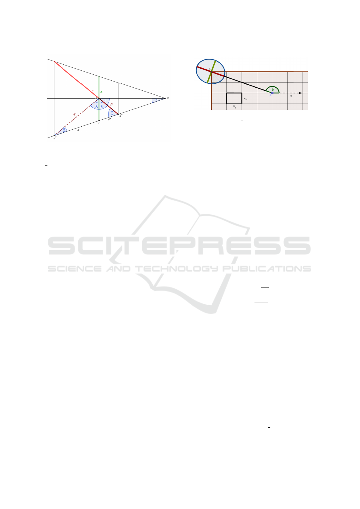
Figure 2: The perpendicular plane segments projected into
one image containing both the minor and major axes of the
ellipse. Using the known angles α and β the searched ratio
a
b
can be computed. Best viewed by rotated figure.
3 ELLIPSE APPROXIMATION
WITH A CIRCLE
One critical part of sphere center estimation is to de-
tect the projection of the sphere in the images. As we
proved in Sec. 2, this shape is a conic section, usually
an ellipse. One particular case is visualized in Fig 1,
where the intersection point of the ellipse axes lands
one of the corners of the image. To robustly fit an
ellipse to image points, either HT or RANSAC (Fis-
chler and Bolles, 1981) has to be applied, but both
methods are slow. The former needs to accumulate
results of the 5D parameter space, and the latter needs
a large iteration number. It principally depends on the
inlier/outlier ratio and the number of parameters to be
estimated. A general ellipse detector needs 5 points,
however, only 3 points are needed for circle fitting.
Therefore, the iteration number of RANSAC can be
significantly reduced by estimating the ellipse with a
circle at the first place.
This section introduces a RANSAC threshold se-
lection process for circle fitting. The threshold should
be larger than the largest distance between the ellipse
and circle contours but this threshold has to be small
enough not to classify to many points as false positive
inliers. The first condition is fulfilled by our defini-
tion of the threshold. Theoretically obtained values
in Fig. 4 show that our approach which based on the
described method in Sec. 3.1 satisfies the second con-
dition as well.
Therefore, one of the novelty in this paper is to
show that circle fitting with higher threshold can be
applied for ellipse fitting. The next section introduces
how this threshold can be selected.
Figure 3: If the ratio of the pixel width and height is u
s
: v
s
,
where u
s
6= v
s
, the ratio
a
b
has to be scaled. This modifica-
tion depends on the pixel scaling factors u
s
, v
s
and the angle
θ between the axis x and the main axis of the ellipse.
3.1 Threshold Selection for Circle
Fitting
Circle model is a rough approximation for ellipses in
robust RANSAC-based (Fischler and Bolles, 1981)
fitting. Although the error threshold for the inlier se-
lection has a paramount importance, manual classifi-
cation is difficult. Basically, this threshold is needed
because of the noise in datapoints. The main idea is
that ellipses can be considered as noisy circles. Real-
istic camera setups confirm this assumption because if
the spherical target is not too close to the image plane,
then the ratio of the ellipse axes will be close to one.
This is convenient in spite of the most extreme visible
position: when the ellipse is as far as possible from
the principal point: near one of the image corners as
it is visualized in Fig. 1.
We propose an adaptive solution to find threshold
t based on the ratio s of the minor and major axes, de-
noted by a and b. In our algorithm, the coherence of
the variables is defined as s =
R+t
R−t
, where R is the ra-
dius of the actually fitted circle in the image. Hence,
the searched variable is t =
(s−1)R
s+1
. Because of realis-
tic simulation, we have to add the noise in pixels.
The discussed 3D problem is visualized in Fig. 1
where not the whole ellipse is fall into the area of the
image. Because of the main goal is to estimate s, two
angles has to be defined: angle α between the axis of
the cone and the image plane and angle β between a
generator of the cone and the axis of the cone. To find
this two angles, consider the two plane segments of
the cone which contain the axis of the cone and ei-
ther the minor or the major axis of the ellipse. The
2D combined visualization is pictured in Fig. 2. This
two views are perpendicular to each other because the
axes of the ellipse are perpendicular. The figure shows
that the minor axis (green) and the axis of the cone
are also perpendicular. If the ellipse center gets fur-
ther from the principal point, then α is smaller and the
difference between a and b steadily increases as it is
seen in Fig. 2. However, if α =
π
2
, the major axis is
also perpendicular to the axis of the cone: this is the
VISAPP 2020 - 15th International Conference on Computer Vision Theory and Applications
492

special case, when a = b and the projection is a circle
which center is the principal point.
First, the vectors and distances have to be de-
fined which determinate α and β. The 2D coordi-
nates of the intersection point X of the ellipse axes
in the image is denoted by
u v
T
, the camera posi-
tion is C =
0 0 0
T
and the distance of the im-
age plane to the camera in the camera coordinate
system is Z = 1. The 3D coordinates of X become
X = ZK
−1
u v 1
T
= Z
h
u−u
0
f
u
v−v
0
f
v
1
i
T
.
The angle α between the axis of the cone and the im-
age plane is determined by two vectors: the direction
vector from X to C, and the vector from X to the prin-
cipal point P = [0,0, f ]
T
, because it is known that the
line of the main axis of the conic section contains the
principal point of the image. The vector coordinates
become
v = XC =Z
u
0
−u
f
u
v
0
−v
f
v
−1
, p = XP = f
u
0
−u
f
u
v
0
−v
f
v
0
.
(3)
Angle α between image plane and cone axis is the
angle between vectors v and p.
Similarly, the angle between the generator and the
axis of the cone depends on the distance of the sphere
center to the camera d =
O − C
and the radius of
the sphere r, shown in Fig. 2. In our approach, r is
given, however, d is undefined because of the varying
position of the sphere. The distance is estimated using
the focal length, the radius of the sphere and the ra-
dius of the fitted ellipse: d =
r f
R
. Considering the two
scalars d and r, the angle becomes β = arcsin(r/d).
The searched ratio can be estimated using the an-
gles α and β and the special properties of the pro-
jections as it is discussed in (Hajder et al., 2020):
a/b =
s
α
c
2
β
/
s
2
α
c
2
β
− c
2
α
s
2
β
.
However, the pixels can be scaled horizontally and
vertically as it is visualized in Fig. 3. The ratio s
depends on this scaling factors u
s
, v
s
and the angle θ
between the direction vector x =
1 0 0
T
along
axis x and the main axis a of the ellipse. Thus, θ is
the angle between vectors −v and x. After applying
elementary trigonometrical expressions, the modified
scale becomes
s =
s
α
c
2
β
s
2
α
c
2
β
− c
2
α
s
2
β
s
u
2
s
c
2
θ
+ v
2
s
s
2
θ
u
2
s
s
2
θ
+ v
2
s
c2
θ
. (4)
Then the RANSAC threshold t =
(s−1)R
s+1
can be com-
puted using the detected circle radius R and the calcu-
lated ratio s.
Figure 4: Estimated RANSAC threshold with varying depth
(top) and varying distance from the principal point in the
image plane (bottom) in case of Blensor tests (left), Carla
tests (middle) and real word tests (right). Red colored part
of the curves in the first row denotes the range of the ap-
plied values in the tests based on the measured depth of the
spheres.
Fig. 4 shows the validation of the automatic
RANSAC threshold estimation with varying depth of
the sphere center and with varying distance between
the ellipse center and the principal point in the im-
age plane in three different test environments, which
are detailed in Sec. 5. The red curve segments show
the range of the applied thresholds in our tests. The
thresholds are realistic and successfully applied in our
ellipse detection method.
4 PROPOSED ALGORITHMS
In this section, the proposed algorithms for spatial
sphere estimation is overviewed. Basically, the esti-
mation consists of two parts: the first one finds the
contours of the ellipse in the image, the second part
determines the 3D location of the sphere correspond-
ing to the ellipse parameters. Simply speaking, the
2D image processing task has to be solved first, then
3D estimation of the location is achieved.
4.1 Ellipse Detector
The main challenge for ellipse estimation is that a
real image may contain many contour lines that are
independent of the observed sphere. There are sev-
eral techniques to find an ellipse in the images as it is
overviewed in the introduction.
Our ellipse fitting method is divided into several
subparts: (i) Edge points are detected in the images.
(ii) The largest circle is found in the processed image
by RANSAC-based (Fischler and Bolles, 1981) circle
fitting on the edge points. (iii) Then the edges with
high magnitude around the selected circle is collected.
(iv) Finally, another RANSAC (Fischler and Bolles,
Automatic Estimation of Sphere Centers from Images of Calibrated Cameras
493

1981)-cycle is run in order to robustly estimate the
ellipse parameters.
Edge Point Detection. RANSAC-based algo-
rithms (Fischler and Bolles, 1981) usually work on
data points. For this purpose, 2D points from edge
maps are retrieved. The Sobel operator (Kanopoulos
et al., 1988) is applied for the original image, then
the strong edge points, i.e. points with higher edge
magnitude than a given threshold, are selected. The
edge selection is based on edge magnitudes, however,
edge directions are also important as the tangent
directions of the contours of ellipses highly depend
on the ellipse parameters. Finally, the points are
made sparser: if there are more strong points in a
given window, only one of those are kept.
Circle Fitting. This is the most critical substep of
the whole algorithm. As it is proven in Sec. 3.1,
the length of the two principal axes of the ellipse
is close to each other. As a consequence, a circle-
fitting method can be applied, and the threshold for
RANSAC, overview in Sec. 3.1 has to be set. The
main challenge for a real application is that only mi-
nority of the points are related to the circle. As it is
pictured in the left image of Fig. 5, only 5 − 10% of
the points can be considered as inliers for circle fit-
ting. Therefore, a very high repetition number is re-
quired for RANSAC. In our practice, millions of iter-
ations are set to obtain acceptable results for real or
realistic test cases.
An important novelty of our circle detector is that
the edge directions are also considered: edge direc-
tions of inliers must be orthogonal to the tangent of
the circle curve.
Collection of Strong Edge Points. The initial cir-
cle estimation yields only a preliminary estimation.
For the final estimation, the points are relocated. For
this purpose, the proposed algorithm searches the
strongest edge points along radial direction. An ex-
ample for the candidate points are visualized in the
center image of Fig. 5.
Final Ellipse Fitting. The majority of the obtained
points belong to the ellipse. However, there can be in-
correct points, effected by e.g. shadows or occlusion.
Therefore, robustification of the final ellipse fitting
is a must. Standard RANSAC (Fischler and Bolles,
1981)-based ellipse fitting is applied in our approach.
We select the method of Fitzgibbon et al. (Fitzgib-
bon et al., 1999) in order to estimate a general ellipse.
A candidate ellipse is obtained then for each circle.
Fourth plot of Fig. 5 shows the candidate ellipses on
the left. There are many ellipses around the correct
solutions, the similar ellipses have to be found: the
final parameters are selected as the average of those.
An example for the final ellipse is visualized in the
right picture of Fig. 5.
4.2 3D Estimation
When the ellipse parameters are estimated, the 3D lo-
cation of the sphere can be estimated as well if the
radius of the sphere is known. All points and the cor-
responding tangent lines of the ellipse in conjunction
with the camera focal points determine tangent planes
of the ellipse. If there is an ellipse, represented by
quadratic equation Ax
2
+ Bxy +Cy
2
+ Dx + Ey + F =
0, it can be rewritten into matrix form if the points are
written in homogeneous coordinates as
x y 1
A
B
2
D
2
B
2
C
E
2
D
2
E
2
F
x
y
1
= 0
The inner matrix, denoted by T in this paper, de-
termines the ellipse. The tangent line l at location
[x y]
T
can be determined by l = T
x y 1
T
as
it is discussed in (Hartley and Zisserman, 2003). Then
the tangent plane of the sphere, corresponding to this
location, can be straightforwardly determined.
The tangent plane of the sphere is determined by
the focal point C. Two of its tangent vectors are rep-
resented by the tangent direction l of the ellipse in the
image space, and the vector
CP. The plane normal is
the cross product of the two tangent vectors.
If a point and the normal, denoted by p
i
and n
i
, re-
spectively, of the tangent plane are given, the distance
of the sphere center with respect to this plane is the
radius r itself. If the length of the normal is unit, in
other words n
T
i
n
i
= 1, the distance can be written as
r = n
T
i
(p
i
− x
0
), where x
0
is the center of the sphere,
that is the unknown vector of the problem. Each tan-
gent plane gives one equation for the center. If there
are three tangent planes, the location can be deter-
mined. In case of at least four planes, the problem
is over-determined. The estimation is given via an in-
homogeneous linear system of equations as follows:
n
T
1
n
T
2
.
.
.
n
T
N
x
0
=
n
T
1
p
1
− r
n
T
2
p
2
− r
.
.
.
n
T
N
p
N
− r
(5)
For the over-determined case, the pseudo-inverse of
the matrix has to be computed and multiplied with
the vector on the right side as the problem is an inho-
mogeneous linear one.
VISAPP 2020 - 15th International Conference on Computer Vision Theory and Applications
494
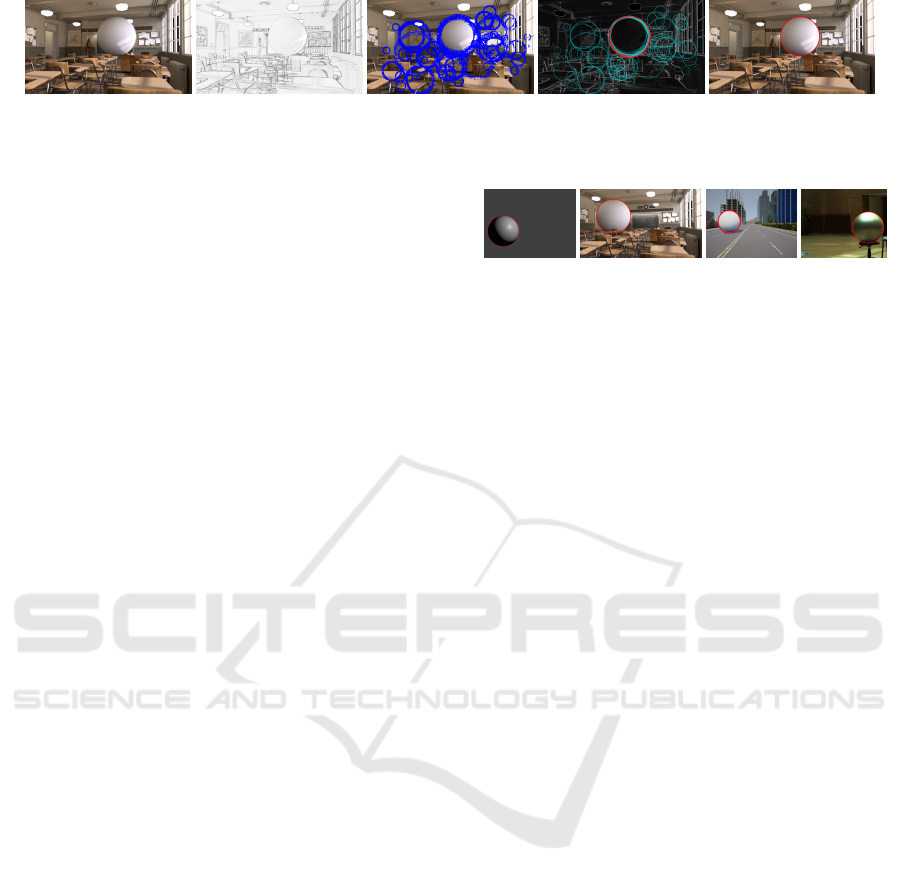
Figure 5: From left to right: (1) Original image generated by Blender. (2) Edge magnituded after applying the Sobel operator.
(3) Candidate points for ellipse fitting. After edge-based circle fitting, the strongest edge points are selected radially for the
candidate circles. (4) Candidate ellipses. Red color denotes the circle with the highest score. (5) Final fitted ellipse.
Numerical Optimization. As the 3D estimation of
the sphere center, defined in Eq. 5, minimizes the
distances in 3D between sphere center and tangent
planes, it is not optimal since the detection error ap-
pears in the image space. Therefore, we apply finally
numerical optimization for estimating the sphere cen-
ter. Initial values for the final optimization are given
by the geometric minimization, then the final solution
is obtained by a numerical optimization. Levenberg-
Marquardt technique is used in our approach.
5 EXPERIMENTS
We have tested the proposed ellipse fitting algorithm
both on three different testing scenarios:
Synthesized Test. In order to test the accuracy and
numerical stability of the algorithms, we have tested
the proposed fitting and 3D estimation algorithms on
a synthetic environment. We have selected Octave
for this purpose. As the 3D models are generated by
the testing environment, quantitative evaluation can
be carried out. The weak-point of the full synthetic
test is that only point coordinates are generated, there-
fore our image-processing algorithm cannot be tested.
Semi-synthetic Test. Semi-synthetic tests extend
the full-synthetic one by images. There are rendering
tools, applied usually for Computer Graphics (CG)
applications, that can generate images of a know vir-
tual 3D scene. We have used Blender as it is one
of the best open-source CG tools and can produce
photo-realistic images. As the virtual 3D models are
known, ground truth sphere locations as well as cam-
era parameters can be retrieved from the tool, there-
fore quantitative evaluation of the algorithms is possi-
ble. The calibration of different devices is very im-
portant for autonomous system, therefore we have
tried the proposed methods for an autonomous sim-
ulator. We selected an open-source simulator, called
CARLA, for this purpose.
Real Test. Even the most accurate CG tools can-
not generate full-realistic images, therefore real test-
ing cannot be neglected. The GT data in these test are
obtained using our novel sphere fitting algorithm, de-
Figure 6: Images for testing. From left to right: (i) Simple
Blender image, (ii) classroom scene rendered by Blender,
(iii) Carla street-view, (iv) a real photo. Detected ellipses
visualized by red.
signed for LiDAR data processing (T
´
oth. and Hajder.,
2019), and by LiDAR-camera calibration.
Synthetic Tests. Synthetic test was only con-
structed in order to validate that the formula, given
in Eq. 5, is correct. For this purpose, a simple syn-
thetic testing environment was implemented in Oc-
tave. Camera parameters as well as the ground-
truth (GT) sphere parameters were randomly gener-
ated, ellipse parameter was computed by projecting
the points into the camera image as it is overviewed
in Section 2.
Conclusion of Synthetic Test. It was successfully val-
idated that Eq. 5 is correct, the Ground-Truth (GT)
sphere parameters can always be exactly retrieved.
Semi-synthetic Tests. The semi-synthetic tests in-
clude virtual scenes containing simple shaded
spheres. The images are generated by the well-known
free and open source 3D creation suite Blender. We
have generated four test images.
Two scenes are generated by Blender. The first
contains only a single sphere with Phong-shading
only. (Left image of Fig. 6). This is considered
as an easier test case, because the images contain
only a single ellipse. The second scene, pictured in
the second image of Fig. 6, is the well-known class-
room scene which is widely used in computer graph-
ics papers. The scene contains several objects and a
sphere. Therefore, the synthetic images are rich in
edges which makes the detectors work harder.
Since the application of these algorithm for
LiDAR-camera calibration is also important, one ad-
ditional scene is rendered by the CARLA simulator.
This scene contains a typical driving simulation with
an additional sphere on the road. An example is visu-
alized in the third image of Fig. 6.
Real Tests. The first important task for a realistic
test is to find a large sphere. We have selected a
Automatic Estimation of Sphere Centers from Images of Calibrated Cameras
495
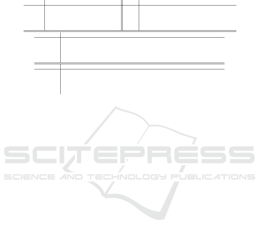
Table 1: Test results for the synthetic and real-world tests. Top rows with the numbers mark the test cases for each test
environments (Blensor, Classroom, Carla and Real), The results are measured Euclidean error between the GT and estimated
ellipse centers by the applied methods. The notations are : Prop. = Proposed method, FAE = FastAndEffective, RHS =
Random Hough Transform, HQ = HighQuality and FI = FastInvariant.
Blensor 1 2 3 4 Real 1 2 3 4 5
Prop. 0.6463 0.0100 0.0372 0.2327 Prop. 0.9115 1.1317 1.7169 0.8702 0.4443
FAE 0.0660 0.1087 0.0601 1.7892 FAE 0.6926 0.2386 0.1566 0.1618 -
RHS 0.7831 0.0537 0.0396 0.1907 RHS 0.6449 0.3330 0.3781 0.1667 0.7859
HQ 0.0516 0.0527 0.0135 0.0263 HQ 0.5231 0.4587 0.3239 0.1734 -
FI
0.0660 0.1087 0.0601 1.7892 FI 0.6926 0.2386 0.1566 0.1618 -
Classroom 1 2 3 4 5 6 7 8
Prop. 0.016 0.0213 0.0302 - 0.2094 - 0.0555 -
FAE 0.0168 0.0168 0.0682 0.0553 - 0.0985 0.1650 -
RHS 0.0689 0.0689 0.1698 0.1165 0.6551 0.41658 7.8553 0.0574
HQ 0.0141 0.0141 0.0037 0.0058 0.0571 0.0056 0.03422 0.0081
FI 0.0168 0.0168 - 0.0553 - 0.0985 0.1650 -
Carla 1 2 3 4 5 6 7 8
Prop. 0.2993 - 1.5381 2.6420 0.3870 1.4974 3.1761 0.55548
FAE - 0.1846 0.1038 2.2196 0.1074 0.6769 0.5710 0.2690
RHS 0.2260 2.17628 1.8085 0.8335 1.0599 0.3954 0.0733 0.32469
HQ 0.0586 0.0486 0.0434 0.0740 0.0933 0.0836 0.1260 0.0391
FI - 0.1846 0.1038 2.2196 0.1074 0.4107 0.5710 -
gymnastic plastic ball for this purpose, with a radius
of 30cm. The images were taken by an iCube cam-
era, whose intrinsic parameters were calibrated using
the chessboard-based calibration method of OpenCV.
Then radial distortion was removed, and the algo-
rithms were run with camera parameters f
u
= f
v
=
4529 (focal length; optics have narrow field of view),
u
0
= 659, v
0
= 619. (principal point; camera sen-
sor resolution is 1280 × 1024). Right image of Fig. 6
shows an example image with detected ellipse.
5.1 Evaluation
The proposed ellipse detector is compared to four
State-of-the-Art (SoA) methods. The error of the
methods measured as the Euclidean distance between
the GT spatial sphere centers and the estimated ones
calculated from the ellipse parameters.
In the real-world tests, the GT is obtained by fit-
ting a sphere to the LiDAR data using our novel
method (T
´
oth. and Hajder., 2019) that is tailored for
LiDAR datapoints. Finally, the sphere centers are
transformed from the LiDAR coordinate system to the
camera coordinate system. The GT data in the syn-
thetic tests are obtained from the testing environment.
Four SoA are compared to the proposed method.
These are as follows: FastAndEffective: (Fornaciari
et al., 2014) proposed a method that can be used
for real-time ellipse detection. First, arch groups are
formed from the Sobel derivatives, then the ellipse pa-
rameters are estimated. The main problem with this
method is the large number of parameters, which have
to be tuned for each image sequence individually.
Random Hough Transform (RHT): The method in-
troduced by (Basca et al., 2005) reduced the compu-
tation time of the HT by randomization. The method
achieves lower detection accuracy, since it consid-
ered only the edge point positions, not their gradi-
ent. HighQuality: (Lu et al., 2020) proposed this
method, which results high quality ellipse parameters.
They generate arcs from Sobel or Canny edge detec-
tors, and several properties of these arcs are exploited,
e.g. overall gradient distribution, arc-support direc-
tions or polarity. This methods need three parame-
ters to be tuned for each test sequence. FastInvari-
ant: (Jia et al., 2016) trade off accuracy for further
speed improvements. Their method removes straight
arcs based on line characteristic and obtains ellipses
by conics.
Table 1 shows the results of both the synthetic and
real-world tests. The rows containing the integer val-
ues are the different image indices in the same test en-
vironment, and the Euclidean error is shown for every
method. In some of the cases, the methods were not
able to find the right ellipses in the images, even after
careful parameter tuning. In these cases, the error of
the method is not presented. The accuracy of the pro-
posed method, denoted by the rows beginning with
Prop., is comparable to the SoA. The best methods is
clearly the HighQuality in all test cases, however, it
was not able to find any ellipse in the 5-th image of
the real-world test. While RHS achieves the worst ac-
curacy, the FastInvariant and FastAndEffective meth-
ods have almost the same results. RHS needs to know
the approximated size of the major axis and the ra-
tio between the minor and major axis of the ellipse
in pixels. The latter two methods require more than
eight parameters to be set. Even though the proposed
method does not achieve significantly better results
then the others, it is the only completely parameter-
free, thus fully automatic, method.
VISAPP 2020 - 15th International Conference on Computer Vision Theory and Applications
496

6 CONCLUSIONS
This paper proposes a novel 3D location estimation
pipeline for spheres. It consists of two steps: (i) the
ellipse is estimated first, (ii) then the spatial location
is computed from the ellipse parameters, if the ra-
dius of the sphere is given and the cameras are cal-
ibrated. Our ellipse detector is accurate as it is vali-
dated by the test. The main benefit of our approach is
that it is fully automatic as all parameters, including
the RANSAC (Fischler and Bolles, 1981) threshold
for circle fitting, can adaptively be set in the imple-
mentation. To the best of our knowledge, our second
method, i.e. the estimator for surface location, is a
real novelty in 3D vision. The main application area
of our pipeline is to calibrate digital cameras to Li-
DAR devices and depth sensors.
ACKNOWLEDGEMENTS
T. T
´
oth and Z. Pusztai were supported by the project
EFOP-3.6.3-VEKOP-16-2017-00001: Talent Man-
agement in Autonomous Vehicle Control Technolo-
gies, by the Hungarian Government and co-financed
by the European Social Fund. L. Hajder was sup-
ported by the project no. ED 18-1-2019-0030: Ap-
plication domain specific highly reliable IT solutions
subprogramme. It has been implemented with the
support provided from the National Research, Devel-
opment and Innovation Fund of Hungary, financed
under the Thematic Excellence Programme funding
scheme.
REFERENCES
Arun, K. S., Huang, T. S., and Blostein, S. D. (1987). Least-
squares fitting of two 3-D point sets. PAMI, 9(5):698–
700.
Basca, C. A., Talos, M., and Brad, R. (2005). Randomized
hough transform for ellipse detection with result clus-
tering. EUROCON 2005”, 2:1397–1400.
Canny, J. F. (1986). A computational approach to edge
detection. IEEE Trans. Pattern Anal. Mach. Intell.,
8(6):679–698.
Chia, A. Y. S., Rahardja, S., Rajan, D., and Leung, M. K.
(2011). A split and merge based ellipse detector with
self-correcting capability. IEEE Trans. Image Pro-
cessing, 20(7):1991–2006.
Duda, R. O. and Hart, P. E. (1972). Use of the hough trans-
formation to detect lines and curves in pictures. Com-
mun. ACM, 15(1):11–15.
Fischler, M. and Bolles, R. (1981). RANdom SAmpling
Consensus: a paradigm for model fitting with appli-
cation to image analysis and automated cartography.
Commun. Assoc. Comp. Mach., 24:358–367.
Fitzgibbon, A., Pilu, M., and Fisher, R. (1999). Direct Least
Square Fitting of Ellipses. IEEE Trans. on PAMI,
21(5):476–480.
Fornaciari, M., Prati, A., and Cucchiara, R. (2014). A fast
and effective ellipse detector for embedded vision ap-
plications. Pattern Recogn., 47(11):3693–3708.
Geiger, A., Moosmann, F., Car, O., and Schuster, B. (2012).
Automatic camera and range sensor calibration using
a single shot. In IEEE International Conference on
Robotics and Automation, ICRA, pages 3936–3943.
Hajder, L., T
´
oth, T., and Pusztai, Z. (2020). Automatic es-
timation of sphere centers from images of calibrated.
Arxiv, available online.
Hartley, R. I. and Zisserman, A. (2003). Multiple View Ge-
ometry in Computer Vision. Cambridge Univ. Press.
Ji, Q. and Hu, R. (2001). Camera self-calibration from el-
lipse correspondences. Proceedings 2001 ICRA. IEEE
International Conference on Robotics and Automation
(Cat. No.01CH37164), 3:2191–2196 vol.3.
Jia, Q., Fan, X., Luo, Z., Song, L., and Qiu, T. (2016). A
fast ellipse detector using projective invariant pruning.
IEEE Transactions on Image Processing, PP.
Kanopoulos, N., Vasanthavada, N., and Baker, R. L. (1988).
Design of an image edge detection filter using the
sobel operator. IEEE Journal of solid-state circuits,
23(2):358–367.
Kim, E., Haseyama, M., and Kitajima, H. (2002). Fast and
robust ellipse extraction from complicated images. In
IEEE Information Technology and Applications.
Kiryati, N., Eldar, Y., and Bruckstein, A. M. (1991). A
probabilistic hough transform. Pattern Recognition,
24(4):303–316.
K
¨
ummerle, J., K
¨
uhner, T., and Lauer, M. (2018). Automatic
calibration of multiple cameras and depth sensors with
a spherical target. In International Conference on In-
telligent Robots and Systems IROS, pages 1–8.
Lu, C., Xia, S., Shao, M., and Fu, Y. (2020). Arc-support
line segments revisited: An efficient high-quality el-
lipse detection. IEEE Transactions on Image Process-
ing, 29:768–781.
Park, Y., Yun, S., Won, C., Cho, K., Um, K., and Sim, S.
(2014). Calibration between color camera and 3d lidar
instruments with a polygonal planar board. Sensors,
14:5333–5353.
Proffitt, D. (1982). The measurement of circularity and
ellipticity on a digital grid. Pattern Recognition,
15(5):383–387.
Shin, I.-S., Kang, D.-H., Hong, Y.-G., and Min, Y.-B.
(2011). Rht-based ellipse detection for estimating the
position of parts on an automobile cowl cross bar as-
sembly. Journal of Biosystems Engineering, 36:377–
383.
Tsuji, S. and Matsumoto, F. (1978). Detection of ellipses by
a modified hough transformation. IEEE Trans. Com-
puters, 27(8):777–781.
T
´
oth., T. and Hajder., L. (2019). Robust fitting of geometric
primitives on lidar data. In VISAPP, pages 622–629.
Yuen, H., Illingworth, J., and Kittler, J. (1988). Ellipse de-
tection using the hough transform.
Automatic Estimation of Sphere Centers from Images of Calibrated Cameras
497
