On Nonintrusive Monitoring of Electrical Appliance Load
Via Restricted Boltzmann Machine with Temporal Reservoir
Megumi Fujita
1 a
, Yu Fujimoto
2 b
and Yasuhiro Hayashi
1 c
1
Graduate School of Advanced Science and Engineering, Waseda University, Tokyo, Japan
2
Advanced Collaborative Research Organization for Smart Society, Waseda University, Tokyo, Japan
Keywords:
Nonintrusive Appliance Load Monitoring, Gaussian-Softmax Restricted Boltzmann Machine, Gaussian
Mixture Model, Reservoir Computing.
Abstract:
This study proposes a nonintrusive appliance load monitoring framework for estimation of the power consump-
tions of individual residential appliances by using aggregated total consumption based on Gaussian-softmax
restricted Boltzmann machine with temporal reservoir. The proposed method is expected to estimate the hid-
den states of the appliances well by coding the current situation in the nonlinear temporal dynamics of the
power consumption in the reservoir units so as to estimate the appliance-wise consumptions well. The accu-
racy of the proposed framework is evaluated by using real-world power consumption data sets.
1 INTRODUCTION
The smart electricity meters are currently being pene-
trating for various electric power consumers in many
parts of the world. These smart meters gather power
consumption data with temporally high resolution ba-
sically for billing purposes of electric utilities; data
collected by smart meters are expected to produce a
new social value and play an important role in the
concept of the Internet of Things (Abate et al., 2018).
However, the current smart meter only has the func-
tion of metering total power consumption at the me-
ter installation site, so that many additional sensors
will be required for presenting the appliance-wise
power consumption to encourage the suppression of
nonessential demand behavior. This paper discusses
a method for estimation of the individual appliance
power consumption by utilizing total power consump-
tion data collected by smart meters without requiring
additional sensors.
An estimation task of appliance-wise energy con-
sumption by utilizing information of aggregated load
collected at a single sensor is called the energy dis-
aggregation or the nonintrusive appliance load mon-
itoring (NILM), and has been discussed since the
1990s (Hart, 1992; Leeb et al., 1995; Cole and Al-
a
https://orcid.org/0000-0002-8163-3664
b
https://orcid.org/0000-0001-8475-0535
c
https://orcid.org/0000-0002-4009-4430
bicki, 1998). The most of the early works have
been focused on relatively high frequency data larger
than 1Hz (Hart, 1992; Leeb et al., 1995; Laughman
et al., 2003), and have also focused on the reactive
power or the other characteristics (Hart, 1992; Leeb
et al., 1995; Cole and Albicki, 1998; Laughman et al.,
2003; Lee et al., 2005). Meanwhile, there are sev-
eral other NILM studies focusing on the relatively low
frequency active power data. Powers et al. (1991)
has utilized the active power information stored ev-
ery 15 minutes; they focused on the spike form of
a large load and proposed the rule based energy dis-
aggregation framework. Farinaccio and Zmeureanu
(1999), and Marceau and Zmeureanu (2000) have uti-
lized the active power stored every 16 seconds and
proposed another rule-based approach focusing on
statistics on the appliance running duration. In recent
decade, the idea of factorial hidden Markov model
(FHMM) (Ghahramani and Jordan, 1997) and appli-
cation of matrix factorization technique (Lee and Se-
ung, 1999) have been also applied for energy disag-
gregation task (Kim et al., 2011; Kolter et al., 2010;
Miyasawa et al., 2019), especially by using relatively
low-frequency active power data set. In particular, the
former is an attractive approach in the sense that it
is possible to derive disaggregation results nearly on-
line using data dynamically observed by a smart me-
ter; however, the characteristics in temporal transition
of the appliance load consumption vary greatly de-
pending on the appliance, so the construction of flex-
902
Fujita, M., Fujimoto, Y. and Hayashi, Y.
On Nonintrusive Monitoring of Electrical Appliance Load Via Restricted Boltzmann Machine with Temporal Reservoir.
DOI: 10.5220/0009164109020909
In Proceedings of the 12th International Conference on Agents and Artificial Intelligence (ICAART 2020) - Volume 2, pages 902-909
ISBN: 978-989-758-395-7; ISSN: 2184-433X
Copyright
c
 2022 by SCITEPRESS – Science and Technology Publications, Lda. All rights reserved

ible and appropriate models within the scope of naive
Markov process is generally difficult. In recent years,
the various artificial neural network schemes also
have been widely applied to the NILM task (Kelly
and Knottenbelt, 2015; He and Chai, 2016; Bonfigli
et al., 2018; Mengistu et al., 2019). However, effec-
tive approaches to achieve NILM considering nonlin-
ear temporal behavior of load consumption flexibly is
still under discussion. For a comprehensive survey of
the NILM framework, we refer the readers to Zeifman
and Roth (2011), and Ruano et al. (2019).
In this paper, we propose a framework of the
NILM task based on the Gaussian-softmax restricted
Boltzmann machines (GSRBMs) (Sohn et al., 2011)
trained in a supervised manner for identifying hidden
states of the target appliances; in particular, we in-
troduce the concept of reservoir computing (Chatzis
and Demiris, 2011) as a framework that takes into ac-
count the nonlinear characteristics of temporal load
consumption inherent to each appliance. We also dis-
cuss the proposed framework by experimentally eval-
uating the accuracy of our proposed method using the
real-world data set.
The rest of the paper is organized as follows. In
Section 2, we explain the basic idea of NILM ap-
proach based on the GSRBM used in this paper. In
Section 3, we introduce an idea of reservoir for rep-
resentation of the temporal behavior of the appliance
load. In Section 4, we show the simulation results
of the proposed approach on real-world data sets for
evaluation. Finally, concluding remarks of the study
are given in Section 5.
2 NILM BASED ON GSRBM
The appliance load monitoring discussed in this pa-
per is based on the accumulated active power con-
sumption data set collected at a single meter in a
household every one minute. We assume that data
sets of appliance-wise power consumptions are uti-
lized for learning background states of each appliance
in a supervised-manner. Firstly, a basic tool used in
our approach, i.e. the GSRBM, is briefly introduced.
Then, an approach for NILM based on GSRBMs is
described.
2.1 GSRBM for Estimation of Hidden
States of Appliance Load
Let v
i
∈ R
+
be the power consumed by the appliance i
in a household, and h
i
= {h
i j
} ∈ {0,1}
J
i
indicate the
hidden load states of the appliance i where J
i
repre-
sents the number of possible states of the appliance
i.
We focus on the following type of restricted Boltz-
mann machine (RBM) (Smolensky, 1986),
p(v
i
,h
i
;θ
i
) =
1
Z(θ
i
)
exp(−E(v
i
,h
i
;θ
i
)), (1)
where E(·) is the energy function of the model
with the parameter set θ
i
= {b
v
i
∈ R, b
h
i j
∈ R ( j =
1,. .., J
i
),w
vh
i j
∈ R ( j = 1,. .., J
i
),σ
i
∈ R
+
}, which is
given as follows,
E(v
i
,h
i
;θ
i
) = −
∑
j
v
i
σ
i
w
vh
i j
h
i j
+
(v
i
− b
v
i
)
2
2σ
2
i
−
∑
j
h
i j
b
h
i j
,
(2)
and Z(θ
i
) is the partition function defined as follows,
Z(θ
i
) =
Z
∞
∞
∑
h
i
exp(−E(v,h
i
;θ
i
))dv. (3)
Here, we introduce the following constraint to h
i
,
∑
j
h
i j
≤ 1. (4)
Then, the model is known to be the Gaussian
RBM (Hinton and Salakhutdinov, 2006) with the soft-
max hidden units, so-called Gaussian-softmax RBM
(GSRBM) (Sohn et al., 2011). The conditional prob-
abilities of v
i
is given as follows,
p(v
i
|h
i
;θ
i
)
=
p(v
i
,h
i
;θ
i
)
R
∞
−∞
p(v, h
i
;θ
i
)dv
=
1
q
2πσ
2
i
exp −
(v
i
− b
v
i
− σ
i
∑
j
w
vh
i j
h
i j
)
2
σ
2
i
!
, (5)
and those of h
i
under the condition shown in Eq. (4)
is given as follows,
p(h
i
|v
i
;θ
i
) =
p(v
i
,h
i
;θ
i
)
∑
h
0
i
p(v
i
,h
0
i
;θ
i
)
=
exp

∑
j
h
i j

v
i
σ
i
w
vh
i j
+ b
h
i j


1 +
∑
j
exp

v
i
σ
i
w
vh
i j
+ b
h
i j

. (6)
Note that the condition
R
∞
−∞
p(v;θ
i
)dv = 1 leads the
marginal probability density function of v
i
to the fol-
lowing mixture model (McLachlan and Peel, 2000) of
K = J +1 Gaussians with the shared variance param-
On Nonintrusive Monitoring of Electrical Appliance Load Via Restricted Boltzmann Machine with Temporal Reservoir
903

eter σ
i
,
p(v
i
;θ
i
) =
∑
h
i
p(v
i
,h
i
;θ
i
)
=
J+1
∑
k=1
π
ik
1
q
2πσ
2
i
exp

−
(v
i
− µ
ik
)
2
2σ
2
i

= GMM
K
(v
i
;ψ), (7)
where ψ = {{π
ik
},{µ
ik
},σ
i
} is the transformed pa-
rameter set for the Gaussian mixture model,
π
ik
=



















exp

b
v
i
w
vh
i j
/σ
i
+(w
vh
i j
)
2
/2+b
h
i j

1+
∑
j
exp

b
v
i
w
vh
i j
/σ
i
+(w
vh
i j
)
2
/2+b
h
i j

(k =1, ... ,J)
1
1+
∑
j
exp

b
v
i
w
vh
i j
/σ
i
+(w
vh
i j
)
2
/2+b
h
i j

(k =J+1(= K)),
(8)
is the weight for the mixture, and
µ
ik
=
(
b
v
i
+ σ
i
w
vh
ik
(k = 1,. ..,J)
b
v
i
(k = J + 1(= K)),
(9)
is the mean parameter of the k-th component Gaus-
sian.
In most of the cases, the parameters in this type
of RBMs are derived by using the approximated
maximum-likelihood approach by using sampling
technique, e.g., contrastive divergence learning (Hin-
ton, 2002; Fischer and Igel, 2014); however, the es-
timation of the variance parameter σ
i
of GSRBM by
the contrastive divergence itself is known to be a dif-
ficult task (Hinton, 2012) and it is also known that the
estimation becomes very difficult when estimating the
other parameters under the small variance parameter
σ
i
even if it is fixed.
In this study, we utilize the fact of equivalence be-
tween the GSRBM and the Gaussian mixture model,
which was discussed in Sohn et al. (2011), to avoid
the difficulties in the learning process. In our im-
plementation, the parameter θ
i
is estimated according
to the following steps using the appliance load data
{v
i
(t);t = 1,..., T }:
Step 1: Estimate mixture of K Gaussians with the
shared variance parameter by using the EM algo-
rithm (McLachlan and Krishnan, 1996) to obtain
the following,
ˆ
ψ
i
= argmax
ψ
i
∑
t
logGMM
K
(v
i
(t);ψ
i
). (10)
Step 2: Iterate Step 1 under various K, and se-
lect the plausible number of components from
the viewpoint of the Bayes information criterion
(BIC) (Schwarz, 1978).
Step 3: Determine σ
i
by using the estimated variance
parameter of the Gaussian mixture model with the
plausible K and substitute the remainder parame-
ters in θ
i
for the GSRBM with J
i
= K − 1 hidden
units as follows:
b
v
i
= µ
iK
, (11)
w
vh
i j
=
1
σ
i
(µ
i j
− b
v
i
) ( j = 1,..., J
i
), (12)
b
h
i j
= log
π
i j
π
iK
−
(w
vh
i j
)
2
2
−
1
σ
i
w
vh
i j
b
v
i
( j = 1,..., J
i
). (13)
2.2 NILM via GSRBM
In the NILM process, we focus on the total consump-
tion of the appliances in the household, i.e. v(t) =
∑
i
v
i
(t), and use the GSRBMs learned beforehand by
using appliance-wise time-series load data to estimate
v
i
(t) for each appliance. Assume that the behaviors of
the appliance load are statistically independent, then
the optimizer of the following problem leads to the
plausible appliance states and the appliance load con-
sumptions,
{ ˆv
i
(t),
ˆ
h
i
(t);∀i} = argmax
{v
i
},{h
i
}
∏
i
p(v
i
,h
i
;θ
i
),
= argmax
{v
i
},{h
i
}
∑
i
log p(v
i
,h
i
;θ
i
),
= argmin
{v
i
},{h
i
}
∑
i
E(v
i
,h
i
;θ
i
), (14)
s.t.
∑
i
v
i
= v(t). (15)
In this study, we focus on the absolute errors between
observed load v(t) and the expected appliance load
under possible hidden states {h
i
} without considering
the constraint given in Eq. (15), i.e.,
e(v(t); {h
i
},{θ
i
}) =





v(t)−
∑
i
b
v
i
+σ
i
∑
j
h
i j
w
vh
i j
!





.
(16)
To obtain the suboptimizer of Eq. (14) under the con-
straint Eq. (15), we extract M-smallest sets of {h
i
}
from the viewpoint of e(v(t); {h
i
},{θ
i
}) shown in
Eq. (16), that is written as H
M
(v(t)) in this paper,
and searched the best solution from H
M
(v(t)) accord-
ing to Algorithm 1. When the number of possible
combinations of hidden states is not large, we can set
M =
∏
i
J
i
, so that Algorithm 1 is reduced to the brute
force global optimization approach.
In this basic idea, only the snapshot v(t) in a
one-dimensional data sequence, {v(t);t = 1,..., T },
ICAART 2020 - 12th International Conference on Agents and Artificial Intelligence
904

Algorithm 1: NILM using GSRBM.
Input: {v(t),{θ
i
},H
M
(v(t))}.
Initialize f ← ∞
for {
˘
h
i
} ∈ H
M
(v(t)) do
Derive the minimizer of Eq. (17) by using the downhill simplex method (Nelder and Mead, 1965),
{ ˘c
i
(t)} = argmin
{c
i
}
∑
i
E

exp(c
i
)
∑
i
0
exp(c
i
0
)
v(t),
˘
h
i
;θ
i

. (17)
Substitute ˘v
i
←
exp(˘c
i
)
∑
i
0
exp(˘c
i
0
)
v(t).
Evaluate f ({˘v
i
},{
˘
h
i
}) =
∑
i
E( ˘v
i
,
˘
h
i
;θ
i
).
if f ({˘v
i
},{
˘
h
i
}) < f then
Update f ← f ({˘v
i
},{
˘
h
i
}), { ˆv
i
(t)} ← { ˘v
i
}, and {
ˆ
h
i
(t)} ← {
˘
h
i
}.
Output: { ˆv
i
(t),
ˆ
h
i
(t); ∀i}.
is used for estimating hidden states and load con-
sumptions of the appliances at the timeslice t based
on the GSRBM (i.e. equivalent to the Gaussian mix-
ture model), so that the behavior of hidden units in
RBMs will not reflect the temporal characteristics of
appliance-specific load consumptions. Therefore, in
the next section, we propose to introduce the idea of
reservoir computing (Chatzis and Demiris, 2011) in
order to take into account the dynamics of appliance-
specific and nonlinear load consumption in estimation
of the hidden states for each appliance, and attempt to
improve the accuracy of load monitoring.
3 TEMPORAL RESERVOIR FOR
MODELING STATE
TRANSITION
Here, we introduce the idea of reservoir comput-
ing (Chatzis and Demiris, 2011) to model nonlinear
temporal dynamics in behavior of appliance load. In
this approach, a set of sparsely and randomly con-
nected units, so-called the reservoir, is introduced
for each appliance model; the weights between con-
nected units in reservoir remains unchanged even dur-
ing the learning process. The model discussed here
can be interpreted as a type of temporal reservoir ma-
chine (Schrauwen and Buesing, 2009) using GSRBM,
and is expected to provide a functionality to memorize
the historical transition of the appliance load by non-
linearly coding into the states of the reservoir units.
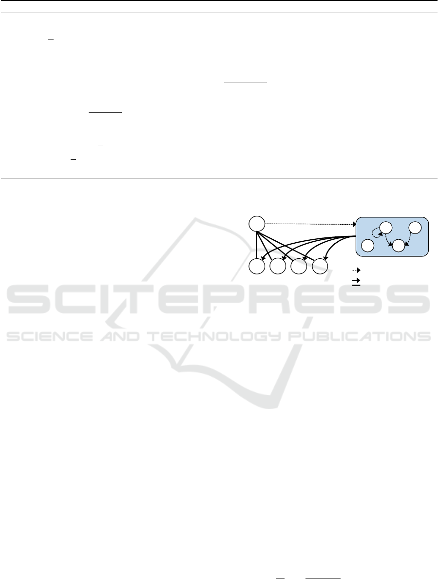
Figure 1 shows the architecture of the GSRBM
with temporal reservoir for modeling state transition
of appliance i. Let r
i
= {r
il
} ∈ (−1,1)
L
be the set of
reservoir units for appliance i, w
rh
il j
∈ R be the weight
!
"
#$%
!"#"$%&'()"*
+",,&)'()"*#
&
"'
(
&
")
( &
"*
(+
-&#&-!."-'()"*#
,
"'
,
")
,
"-
+
.
"/
01
.
"//
11
.
"//
12
.
"/
02
3
"
0
3
"/
2
/"!&)'-0),.1%2
3-0")&,'$2'(#")4',0*0
!
Figure 1: Architecture of the GSRBM with temporal reser-
voir for modeling state transition of appliance i.
from reservoir unit r
il
to hidden unit h
i j
, w
vr
il
∈ R be
the weight from visible unit v
i
to the reservoir unit r
il
,
and W
rr
i
= {w
rr
ilm
} ∈ R
L×L
be the matrix containing the
weight from the reservoir unit r
il
to r
im
. We assume
that the states of the reservoir units at the timeslice
t +1, i.e. {r
il
(t +1)}, are uniquely determined by the
current states {r
il
(t)} and the current appliance load
v
i
(t) as follows,
r
il
(t + 1) = tanh

∑
m
w
rr
iml
r
im
(t) + w
vr
il
v
i
(t)

. (18)
Note that the states of these reservoir units are ex-
pected to represent the current situation over the
historical load transition taking into account the
appliance-specific dynamics of power consumption
{v
i
(t)}.
We focus on the energy function of the original
GSRBM conditioned by the given reservoir units r
i
under the architecture shown in Fig. 1 as follows,
E(v
i
,h
i
| r
i
;φ
i
)
=−
∑
j
w
vh
i j
v
i
σ
i
h
i j
+
(v
i
−b
v
i
)
2
2σ
2
i
−
∑
j,l
w
rh
il j
h
i j
r
il
−
∑
j
h
i j
b
h
i j
,
(19)
On Nonintrusive Monitoring of Electrical Appliance Load Via Restricted Boltzmann Machine with Temporal Reservoir
905

where the parameter φ
i
is given as φ
i
=
{b
v
i
,{b
h
i j
},{w
vh
i j
},{w
rh
il j
},σ
i
}, so that the target
conditional probability distribution p(v
i
,h
i
| r
i
;φ
i
) is
given as follows,
p(v
i
,h
i
| r
i
;φ
i
) ∝ exp(−E(v
i
,h
i
| r
i
;φ
i
)). (20)
Under the same constraint given in Eq. (4), the condi-
tional probabilities of h
i
is described as the following
form,
p(h
i
| v
i
,r
i
;φ
i
)
=
exp

∑
j
h
i j

v
i
σ
i
w
vh
i j
+
∑
l
w
rh
il j
r
il
+ b
h
i j

1 +
∑
j
exp

v
i
σ
i
w
vh
i j
+
∑
l
w
rh
il j
r
il
+ b
h
i j

, (21)
which is affected by the reservoir r
i
.
In our implementation, the parameter φ
i
in the
model shown in Eq. (20) is estimated by the con-
trastive divergence method using the initial GSRBM
parameters derived by the EM algorithm as follows:
Step 1: Select the optimal number of hidden
units J
i
and estimate the GSRBM parameters
{b
v
i
,{w
vh
i j
},{b
h
i j
},σ
i
} as an initial parameter
subset.
Step 2: Initialize {w
vr
il
}, {w
rh
il j
} and W
rr
i
: w
vr
il
is gen-
erated from the continuous uniform distribution in
the range [−0.1,0.1]; w
rh
il j
is initialized by zero;
the five percents of the elements randomly se-
lected in the weight matrix W
rr
i
are set to have
nonzero values also given randomly and scaled so
as to hold ρ(W
rr
i
) < 1 where ρ(W ) is the maxi-
mum absolute eigenvalue of the matrix W .
Step 3: Iteratively update the parameters b
v
i
,
{b
h
i j
},{w
vh
i j
},{w
rh
il j
} using the contrastive diver-
gence (CD-1) method (Hinton, 2002);
b
v
i
← b
v
i
+ε
1
T
T
∑
t=1
(v
i
(t) − ˜v
i
(t)), (22)
b
h
i j
← b
h
i j
+ε
1
T
T
∑
t=1

h
0
i j
(t) −
˜
h
i j
(t)

(∀ j), (23)
w
vh
i j
← w
vh
i j
+ε
1
T
T
∑
t=1

v
i
(t)h
0
i j
(t) − ˜v
i
(t)
˜
h
i j
(t)

(∀ j),
(24)
w
rh
il j
← w
rh
il j
+ε
1
T
T
∑
t=1
r
il
(t)

h
0
i j
(t) −
˜
h
i j
(t)

(∀ j, l),
(25)
where ε is a small positive constant and
h
0
i
(t) = {h
0
i j
(t)} ∼ p(h
i
(t)|v
i
(t),r
i
(t); φ
i
), (26)
˜v
i
(t) ∼ p(v
i
(t)|h
0
i
(t); φ
i
), (27)
˜
h
i
(t) = {
˜
h
i j
(t)} ∼ p(h
i
| ˜v
i
(t),r
i
(t); φ
i
). (28)
In our proposed scheme, the GSRBMs with tem-
poral reservoir are utilized instead of naive GSRBMs
in the NILM process described in Section 2. The es-
timation of plausible states and load consumptions of
the appliances is achieved as
{ ˆv
i
(t),
ˆ
h
i
(t); ∀i} = argmin
{v
i
},{h
i
}
∑
i
E(v
i
,h
i
| r
i
(t); φ
i
),
s.t.
∑
i
v
i
= v(t), (29)
by substituting the energy functions of the models
with reservoir, i.e. {E(v
i
,h
i
| r
i
(t); φ
i
)}, for those of
naive GBRBMs {E(v
i
,h
i
;θ
i
)} in Eq. (15). Note that
in the monitoring process, the reservoir {r
il
(t + 1)}
is affected by ˆv
i
(t), which is the disaggregated load
consumption of the appliance i, and the current states
of the reservoir units according to Eq. (18). The op-
timization problem shown in Eq. (29) can be also
searched by Algorithm 1 using the models with reser-
voir instead of the naive GSRBMs. Since the reser-
voir has the function of coding the nonlinear dynam-
ics and history of the transition of individual appli-
ance load consumption up to the current timeslice t
into L units, this approach is expected to be a way
to handle temporal characteristics relatively flexible
comparing with a model assuming a simple low-order
Markov process of the observed sequence {v
i
(t)} for
each appliance.
4 NUMERICAL EXPERIMENTS
The proposed NILM framework was numerically
evaluated from the viewpoint of estimation accuracy
using real-world data sets collected at ten households.
The data sets were composed of power consumptions
of four appliances, i.e. the refrigerator, the wash-
ing machine, the heater, and the air conditioners, col-
lected every one minute from July 1st to July 7th in
2017. Figure 2 shows an example of the appliance-
wise power consumptions used in the experiments. In
the experimental setup, the NILM approach was eval-
uated by using the sequence of total power consump-
tions of these four appliances collected at one of the
ten households; each appliance model was learned by
using the set of appliance-wise data collected at the
rest of nine households. The evaluation was processed
for all the ten households in a manner of the cross
validation. We especially focus on evaluating the ef-
fectiveness of the reservoir units by comparing with
the scheme based on the naive GBRBMs introduced
in Section 2, and the simple mean prediction algo-
rithm (Kolter and Johnson, 2011) as a benchmark; the
ICAART 2020 - 12th International Conference on Agents and Artificial Intelligence
906

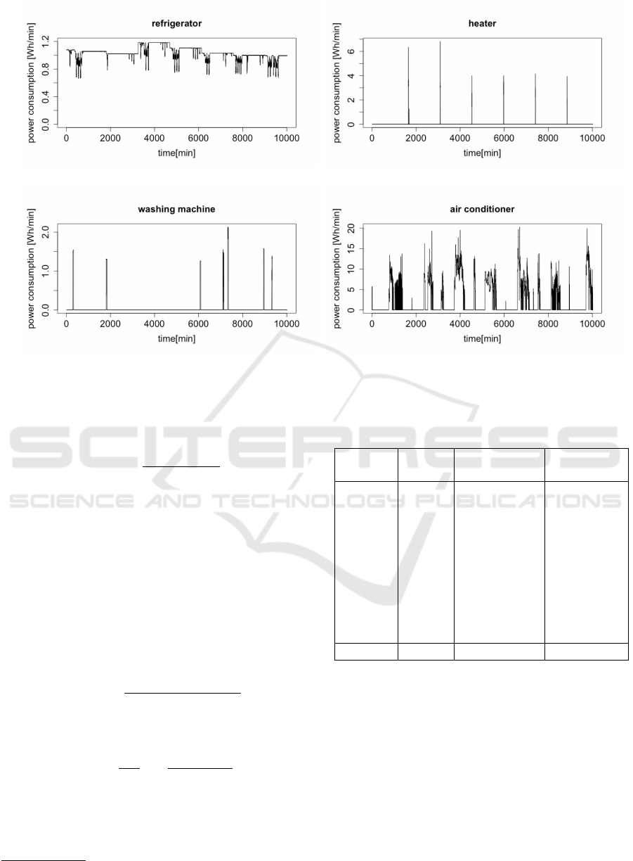
(a) Refrigerator
(b) Washing machine
(c) Heater
(d) Air conditioner
Figure 2: Appliance-wise power consumptions. The input for the NILM task is an aggregated sequence of these consumptions.
latter is given as follows:
ˆv
i
(t) = v(t)
∑
T
t
0
=1
v
(lrn)
i
(t
0
)
∑
T
t
0
=1
v
(lrn)
(t
0
)
, (30)
where v
(lrn)
i
and v
(lrn)
indicate the power consumption
of the appliance i and the total power consumption
in the learning data set, respectively. The number of
hidden units was derived according to the process de-
scribed in Section 3, and given as 12 for air condi-
tioner, five for washing machine, six for refrigerator,
and five for heater, respectively. The number of reser-
voir units was given as L = 100 in this study. The
results of the NILM were evaluated from the view-
point of disaggregation accuracy defined in Kolter and
Johnson (2011),
ACC = 1 −
∑
T
t=1
∑
i
| ˆv
i
(t) − v
i
(t)|
2
∑
T
t=1
v(t)
, (31)
and that of the appliance-wise percentage mean abso-
lute error
1
,
PMAE
i
=
100
T
T
∑
t=1




ˆv
i
(t) − v
i
(t)
v
i
(t)




. (32)
Table 1 shows the comparison results of the NILM
task for ten households. The result shows that the pro-
posed architecture based on the GSRBM with reser-
voir is better than the simple mean approach, nor
1
Note that the PMAE for the power consumption of
home appliances that are used for a short time can be large.
Table 1: Comparison of disaggregation accuracy (ACC).
House Simple GSRBM GSRBM
ID mean w/o reservoir w/ reservoir
1 0.6560 0.9688 0.9691
2 0.6604 0.8866 0.8866
3 0.6339 0.9690 0.9690
4 0.7027 0.9604 0.9608
5 0.5250 0.9418 0.9418
6 0.6055 0.9488 0.9490
7 0.6171 0.9236 0.9239
8 0.5443 0.9599 0.9598
9 0.6275 0.9407 0.9423
10 0.6538 0.9083 0.9083
Average 0.6226 0.9408 0.9411
the ordinary GSRBM in most of the cases. The
results suggest that the proposed architecture pro-
vides a promising NILM framework for handling
nonlinear temporal dynamics in behavior of appliance
load. Figure 3 shows the comparison results of the
appliance-wise percentage mean absolute errors. The
figure suggests that the proposed GSRBMs drastically
reduce the mean absolute errors by comparing with
the simple mean prediction results. Particularly, the
estimation errors of the proposed framework based on
the GSRBM with reservoir tend to be slightly smaller
than those of the ordinary GSRBM, though the results
imply that other approaches may need to be consid-
On Nonintrusive Monitoring of Electrical Appliance Load Via Restricted Boltzmann Machine with Temporal Reservoir
907

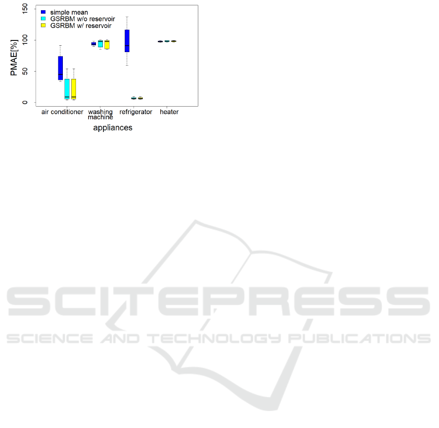
Figure 3: Comparison of appliance-wise percentage mean
absolute errors (PMAE
i
).
ered to reduce the estimation errors of the appliances
that only works occasionally, such as washing ma-
chines and heaters.
5 CONCLUDING REMARKS
In this study, we focused on a nonintrusive appliance
load monitoring scheme based on Gaussian-softmax
RBM, and proposed to introduce the temporal reser-
voir function for the purpose of modeling the nonlin-
ear temporal behavior of the appliance load consump-
tion. The proposed framework was evaluated from the
viewpoint of estimation accuracy by numerical exper-
iments. The experimental results show that the in-
troduction of the reservoir tends to improve the es-
timation accuracy of the appliance-wise energy con-
sumption. Thus, the proposed architecture will be a
promising framework for handling nonlinear tempo-
ral dynamics in appliance load.
Our experimental results suggested that an explicit
mechanism is required to further improve the estima-
tion accuracy for the appliances that only work occa-
sionally, such as washing machines and heaters. Ad-
ditionally, we also plan to develop a scheme utilizing
information stored in the reservoir during the NILM
process for the short-term forecast of appliance-wise
electricity consumption, though it remains as a future
work.
ACKNOWLEDGEMENTS
A part of this work was supported by the Japan Sci-
ence and Technology Agency (JST), Core Research
for Evolutional Science and Technology (CREST)
Program, under Grant JPMJCR15K5.
REFERENCES
Abate, F., Carrat
`
u, M., Liguori, C., Ferro, M., and Paciello,
V. (2018). Smart meter for the IoT. In 2018 IEEE In-
ternational Instrumentation and Measurement Tech-
nology Conference: Discovering New Horizons in In-
strumentation and Measurement, Proceedings, pages
1–6.
Bonfigli, R., Felicetti, A., Principi, E., Fagiani, M., Squar-
tini, S., and Piazza, F. (2018). Denoising autoencoders
for Non-Intrusive Load Monitoring: Improvements
and comparative evaluation. Energy and Buildings,
158:1461–1474.
Chatzis, S. P. and Demiris, Y. (2011). Echo state Gaus-
sian process. IEEE Transactions on Neural Networks,
22(9):1435–1445.
Cole, A. I. and Albicki, A. (1998). Algorithm for non-
Intrusive Identification of Residential Appliances. In
I, volume III, pages 338–341.
Farinaccio, L. and Zmeureanu, R. (1999). Using a Pattern
Recognition Approach to Disaggregate the Total Elec-
tricity COnsumption in a House into the Major End-
Uses. Energy and Buildings, 30:245–259.
Fischer, A. and Igel, C. (2014). Training restricted Boltz-
mann machines: An introduction. Pattern Recogni-
tion, 47(1):25–39.
Ghahramani, Z. and Jordan, M. I. (1997). Factorial Hidden
Markov Models. Machine Learning, 29:245–273.
Hart, G. W. (1992). Nonintrusive Appliance Load Monitor-
ing. Proceedings of the IEEE, 80(12):1870–1891.
He, W. and Chai, Y. (2016). An Empirical Study on En-
ergy Disaggregation via Deep Learning. In 2nd In-
ternational Conference on Artificial Intelligence and
Industrial Engineering, volume 133, pages 338–342.
Hinton, G. E. (2002). Training Products of Experts by Mini-
mizing Contrastive Divergence. Neural Computation,
14(8):1771–1800.
Hinton, G. E. (2012). A practical guide to training restricted
Boltzmann machines. In Neural Networks: Tricks
of the Trade, pages 599–619. Springer Berlin Heidel-
berg.
Hinton, G. E. and Salakhutdinov, R. R. (2006). Reduc-
ing the Dimensionality of Data with Neural Networks.
Science, 313:504–507.
Kelly, J. and Knottenbelt, W. (2015). Neural NILM: Deep
Neural Networks Applied to Energy Disaggregation.
In BuildSys@SenSys.
Kim, H., Marwah, M., Arlitt, M., Lyon, G., and Han, J.
(2011). Unsupervised Disaggregation of Low Fre-
quency Power Measurements. In SIAM Conference
on Data Mining 2011, pages 747–758.
Kolter, J. Z., Batra, S., and Ng, A. Y. (2010). Energy Disag-
gregation via Discriminative Sparse Coding. In Neu-
ral Information Processing Systems.
Kolter, J. Z. and Johnson, M. J. (2011). REDD: A Pub-
lic Data Set for Energy Disaggregation Research. In
Workshop on Data Mining Applications in Sustain-
ability.
ICAART 2020 - 12th International Conference on Agents and Artificial Intelligence
908

Laughman, C., Lee, D., Cox, R., Shaw, S., Leeb, S., Nor-
ford, L., and Armstrong, P. (2003). Advanced Non-
intrusive Monitoring of Electric Loads. IEEE Power
and Energy Magazine, pages 56–63.
Lee, D. D. and Seung, H. S. (1999). Learning the parts of
objects by non-negative matrix factorization. Nature,
401(6755):788–791.
Lee, K. D., Leeb, S. B., Norford, L. K., Armstrong, P. R.,
Holloway, J., and Shaw, S. R. (2005). Estimation of
Variable-Speed-Drive Power Consumption From Har-
monic Content. IEEE Transactions on Energy Con-
version, 20(3):566–574.
Leeb, S. B., Shaw, S. R., and James L. Kirtley, J. (1995).
Transient Event Detection in Spectral Envelope Esti-
mates for Nonintrusive Load Monitoring. IEEE Trans-
actions on Power Delivery, 10(3):1200–1210.
Marceau, M. L. and Zmeureanu, R. (2000). Nonintrusive
Load Disaggregation Computer Program to Estimate
the Energy Consumption of Major End Uses in Res-
idential Buildings. Energy Conversion and Manage-
ment, 41:1389–1403.
McLachlan, G. and Peel, D. (2000). Finite Mixture Models.
Wiley.
McLachlan, G. J. and Krishnan, T. (1996). The EM Algo-
rithm and Extensions. Wiley-Interscience.
Mengistu, M. A., Girmay, A. A., Camarda, C., Acquaviva,
A., and Patti, E. (2019). A Cloud-Based On-Line Dis-
aggregation Algorithm for Home Appliance Loads.
IEEE Transactions on Smart Grid, 10(3):3430–3439.
Miyasawa, A., Fujimoto, Y., and Hayashi, Y. (2019). En-
ergy disaggregation based on smart metering data via
semi-binary nonnegative matrix factorization. Energy
and Buildings, 183:547–558.
Nelder, J. and Mead, R. (1965). A Simplex Method
for Function Minimization. The Computer Journal,
7(4):308–313.
Powers, J., Margossian, B., and Smith, B. (1991). Using a
Rule-Based Algorithm to Disaggregate End-Use Load
Profiles from Premise-Level Data. IEEE Computer
Applications in Power, 4(2):27–42.
Ruano, A., Hernandez, A., Ure
˜
na, J., Ruano, M., and Gar-
cia, J. (2019). NILM techniques for intelligent home
energy management and ambient assisted living: A
review. Energies, 12(11):1–29.
Schrauwen, B. and Buesing, L. (2009). A hierarchy of re-
current networks for speech recognition. NIPS Work-
shop on Deep Learning for Speech Recognition and
Related Applications, pages 1–8.
Schwarz, G. (1978). Estimating the Dimension of a Model.
Annals of Statistics, 6(2):461–464.
Smolensky, P. (1986). Parallel distributed processing: Ex-
plorations in the microstructure of cognition. In MIT
Press, Cambridge, MA, USA, volume 1, chapter 6,
pages 194–281.
Sohn, K., Jung, D. Y., Lee, H., and Hero, A. O. (2011).
Efficient learning of sparse, distributed, convolutional
feature representations for object recognition. In Pro-
ceedings of the IEEE International Conference on
Computer Vision, pages 2643–2650.
Zeifman, M. and Roth, K. (2011). Nonintrusive Appliance
Load Monitoring: Review and Outlook. IEEE Trans-
actions on Consumer Electronics, 57(1):76–84.
On Nonintrusive Monitoring of Electrical Appliance Load Via Restricted Boltzmann Machine with Temporal Reservoir
909