Study on the Average Size of the Longest-Edge Propagation Path for
Triangulations
Oliver-Amadeo Vilca Huayta
1 a
and Mar
´
ıa-Cecilia Rivara
2 b
1
Departamento de Ingenier
´
ıa de Sistemas, Universidad Nacional del Altiplano, Avenida Floral N. 1153, Puno, Peru
2
Departamento de Ciencias de la Computaci
´
on, Universidad de Chile, Santiago, Chile
Keywords:
Average LEPP Size, Longest-Edge Propagating Path (LEPP), Triangulation Refinement.
Abstract:
For a triangle t in a triangulation τ, the “longest edge propagating path” Lepp(t), is a finite sequence of
neighbor triangles with increasing longest edges. In this paper we study mathematical properties of the LEPP
construct. We prove that the average LEPP size over triangulations of random points sets, is between 2 and 4
with standard deviation less than or equal to
√
6. Then by using analysis of variance and regression analysis
we study the statistical behavior of the average LEPP size for triangulations of random point sets obtained
with uniform, normal, normal bivariate and exponential distributions. We provide experimental results for
verifying that the average LEPP size is in agreement with the analytically derived one.
1 INTRODUCTION
Triangulations are extensively used in a variety of
applications such that finite element analysis, com-
puter graphics, animation, visualization and computer
aided design. Triangulation refinement for adaptive
finite element methods is a process (algorithm) that
for an input set S of target triangles with unacceptable
finite element error, produces a valid refined triangu-
lation (the triangles of S and some neighbor triangles
are refined) such that the triangulation quality is main-
tained throughout the process. Refinement algorithms
based on the longest edge bisection of triangles were
developed for adaptive and multigrid finite element
methods (Rivara, 1984a; Rivara, 1984b), which main-
tain the triangulation quality due to the mathematical
properties of the longest edge bisection of triangles.
Later the LEPP construct was introduced and used
in two directions: (1) to reformulate in a simpler and
effective way previous longest edge refinement algo-
rithms, which maintain the quality of the initial trian-
gulation (Rivara, 1997; Bedregal and Rivara, 2014a);
and (2) to develop LEPP Delaunay algorithms for
the quality triangulation of planar straight line graph
(PSLG) geometries, which improve a bad quality tri-
angulation of the input PSLG data (Rivara, 1997;
Bedregal and Rivara, 2014b; Rivara and Rodriguez-
Moreno, 2019).
a
https://orcid.org/0000-0002-5703-790X
b
https://orcid.org/0000-0001-9041-6154
The LEPP algorithms work as follows, given a
target triangle t to be refined / improved, a finite se-
quence of increasing neighbor triangles (where t
i+1
is neighbor of t
i
by the longest edge of t
i
, and the
longest edge of t
i+1
is greater than the longest edge
of t
i
) is computed. This sequence, called Lepp(t), al-
lows finding a local largest edge (terminal edge) in
the mesh shared by a couple of terminal triangles (for
an illustration see Figure 1). Then, over the couple
of terminal triangles, a local refinement operation is
performed, which locally improves the triangulation
quality. The local refinement operations used are ei-
ther the longest edge bisection of the terminal trian-
gles, or the Delaunay insertion of a point selected in
the interior of the terminal triangles (terminal edge
midpoint or centroid of the terminal triangles).
It has been proven that the LEPP algorithms pro-
duce optimal size triangulations due to the improve-
ment properties of the local operations performed in-
side the terminal triangles, which in turn implies that
the average size (number of triangles) of Lepp(t) de-
creases and tends to be 3 as the refinement proceeds
(Bedregal and Rivara, 2014a; Rivara and Rodriguez-
Moreno, 2019).
We should emphasize that the LEPP construct re-
sulted to be an effective and simple tool for mesh im-
provement both in 2D and 3D suitable to be included
in mesh generation software and for parallelization.
Discussions on these issues can be found in (Rivara
and Rodriguez-Moreno, 2019; Balboa et al., 2019).
368
Huayta, O. and Rivara, M.
Study on the Average Size of the Longest-Edge Propagation Path for Triangulations.
DOI: 10.5220/0009162703680375
In Proceedings of the 15th Inter national Joint Conference on Computer Vision, Imaging and Computer Graphics Theory and Applications (VISIGRAPP 2020) - Volume 1: GRAPP, pages
368-375
ISBN: 978-989-758-402-2; ISSN: 2184-4321
Copyright
c
 2022 by SCITEPRESS – Science and Technology Publications, Lda. All rights reserved

In this paper we study the average LEPP size over
static triangulations which are the input meshes re-
quired in different complex applications such those
related with finite element methods. More specifi-
cally, we compute the worst LEPP size, and the av-
erage LEPP size for triangulations of sets of random
points in 2D.
It is important to study the average LEPP size be-
cause this is the most frequent case in the triangula-
tion refinement process. This is similar to what hap-
pens with the Quicksort algorithm, where on the av-
erage case the execution time is optimal n ·log(n) to
sort n items and has better performance than its com-
petitors, but it is bad in the worst case n
2
(Sedgewick
and Wayne, 2011; Sedgewick and Flajolet, 2013).
2 RELATED WORK
Formally, Lepp(t) is defined as follows: for any
triangle t
1
in τ, the longest edge propagating path
(Lepp(t
1
)) is defined as the finite sequence of increas-
ing triangles {t
i
}
n
i=1
such that t
i+1
is the neighbor of
t
i
by its longest edge, and where the longest edge of
t
i+1
is greater than the longest edge of t
i
. The LEPP
path allows to find an associated local largest edge E
(terminal edge) in τ, either shared by two terminal tri-
angles t
n−1
,t
n
, or E being a boundary terminal edge
(longest edge of t
n
). For an illustration see Figure 1,
where AB is an interior terminal edge.
LEPP algorithms (Rivara, 1997; Bedregal and Ri-
vara, 2014a; Bedregal and Rivara, 2014b; Rivara
and Calderon, 2010; Rivara and Rodriguez-Moreno,
2019) proceed as follows: for each target triangle t
to be refined / improved, the longest edge propagat-
ing path (LEPP) is computed to find a couple of ter-
minal triangles sharing a common longest edge AB
(terminal edge) as shown in Figure 1. Then a point is
selected inside the terminal triangles (terminal edge
midpoint or terminal triangles centroid) and inserted
in the mesh either by triangle longest edge bisection
or by Delaunay insertion. The process is repeated un-
til the target triangle is refined.
Note that over the terminal triangles local refine-
ment operations are performed which locally improve
the triangulation quality.
LEPP Bisection Algorihtm. Due to the improve-
ment properties of the iterative longest edge bisec-
tion of triangles, refined triangulations that maintain
the triangulation quality (bounded smallest angle) are
obtained, while the proportion of quality triangles in-
creases as the refinement proceeds. Based on these
properties, it has been proven that optimal size trian-
gulations are obtained (Bedregal and Rivara, 2014a).
Figure 1: Lepp(t
1
) = {t
1
,t
2
,t
3
,t
4
} in triangulations τ allows
to find a local largest edge (terminal edge) AB and a cou-
ple of terminal triangles (t
3
,t
4
) over which refinement / im-
provement operations are performed.
LEPP Delaunay Algorithms. These algorithms pro-
duce quality Delaunay triangulation, based on the De-
launay insertion of special points inside the terminal
triangles (terminal edge midpoint or centroid of the
terminal triangles). For the LEPP centroid algorithm,
termination, and optimal size property were proven.
Furthermore the size of the refined triangulation is al-
most equal independently of the triangle processing
order (Rivara and Rodriguez-Moreno, 2019). In 3-
dimensions a mesh improvement algorithm based on
the extensions of some of these ideas to 3-dimensions
have been also discussed (Balboa et al., 2019).
2.1 On the LEPP Size
In the LEPP algorithms, for each target triangle t
(to be refined or improved) the LEPP computation is
repeatedly performed until the triangle is destroyed.
Thus the number of points inserted to refine / im-
prove triangle t roughly depends on the LEPP size.
For the LEPP algorithms it has been proven that the
average LEPP size is small and tends to be 3 as the re-
finement algorithm proceeds. This was firstly proven
for triangulations obtained by the LEPP bisection al-
gorithm (Bedregal and Rivara, 2014a) and later ex-
tended to the LEPP Delaunay algorithms (Rivara and
Rodriguez-Moreno, 2019).
In this paper we state results on the average LEPP
size for triangulations. Assuming that the probability
of finding a longest edge neighbor in the LEPP path
is p ≥
1
3
, we prove that the average LEPP size is be-
tween 2 and 4. We also present a statistical study over
triangulations of random point sets, showing that the
average LEPP size is in agreement with the theory.
Study on the Average Size of the Longest-Edge Propagation Path for Triangulations
369

3 THEORETICAL STUDY ON
THE AVERAGE LEPP SIZE
3.1 Worst Case on the LEPP Size
In the worst case, the LEPP size is equal to the size of
the triangulation τ, the number of triangles n, which
occurs for the special case where there exists a small-
est triangle t
1
, such that, Lepp(t
1
) covers τ and size of
Lepp(t
1
) is equal to n. For an example see Figure 2.
...
t
1
t
n
t
5
t
3
4
t
t
2
Figure 2: Worst case of the maximum LEPP size (with n
triangles).
Here the average LEPP size is equal to
µ
LEPP
=
n
∑
i=1
Lepp(t
i
)
n
=
n
∑
i=1
i
n
=
n + 1
2
(1)
Note that in this case the average LEPP size in-
creases with n.
3.2 Theoretical Average LEPP Size
Here we calculate the average LEPP size of triangu-
lations. This extends and improves results presented
in (Vilca, 2009; Vilca et al., 2010), the following more
general theorems are formulated in terms of a param-
eter p. In section 4 we also include statistical discus-
sion on empirical results.
Firstly we need to introduce the following defini-
tion:
Definition 1. For any triangle t of longest edge E and
neighbor triangle t
∗
with edges E
∗
1
≥E
∗
2
≥E
∗
3
, we will
say that the neighbor triangle t
∗
by the edge E is of
type A, B, C if the following conditions hold:
- t
∗
is of type A if E = E
∗
3
- t
∗
is of type B if E = E
∗
2
- t
∗
is of type C if E = E
∗
1
Theorem 1. Let τ a triangulation constructed from a
set of random points in 2D, if for any triangle in τ the
probability of having a neighbor triangle of type C is
p, then the average LEPP size is
p+1
p
with standard
deviation equal to
√
1−p
p
, the skewness coefficient is
equal to
2−p
√
1−p
, and the kurtosis coefficient is equal to
p
2
−6p+6
1−p
.
Proof. If for any triangle T
i
the probability of having
a neighboring triangle T
i+1
of type C is p, then, the
probability of having a neighboring triangle of type A
or B is q (where p + q = 1).
It is easy to see that Lepp(T
1
) is an ordered se-
quence of triangles composed of three parts: (i) An
initial triangle T
1
without type because the first tri-
angle does not have a predecessor neighbor triangle.
(ii) Followed indistinctly by zero or more triangles
of type A or B, and (iii) ending with a triangle T
n
of
type C. Then the minimum length of the LEPP is two
(composed of the first triangle without type and the
last type C triangle).
The above sequence corresponds to the geometric
distribution P(n) = q
k
p, where the mean on the aver-
age number of triangles of type A or B is µ =
q
p
, to
which a value 2 should be added, according to items
(i) and (iii) on the number of elements in the LEPP
path. Thus, the average LEPP size is
p+1
p
. Further-
more the variance, third and fourth moments are given
by:
V (G) =
q
p
2
(2)
µ
3
=
q(2 − p)
p
3
(3)
µ
4
=
q(p
2
−9p +9)
p
4
(4)
Finally, from equation 2, the standard deviation of
the average LEPP size is σ =
p
V (G) =
√
1−p
p
, while
the coefficients of skewness and kurtosis are:
Sk =
µ
3
σ
3
=
2 − p
√
1 − p
(5)
Ku =
µ
4
σ
4
−3 =
p
2
−6p +6
1 − p
(6)
Remark Theorem 1 does not consider triangles t
e
with boundary longest edges (Leep(t
e
) = 1). There-
fore, this is indeed a result over an infinite mesh.
Theorem 2. Let τ be a triangulation constructed from
a set of random points in 2D and let µ
LEPP
be the av-
erage LEPP size, then 2 ≤ µ
LEPP
≤ 4 with standard
deviation between 0 and
√
6, assuming that for any
triangle in τ the probability of having a neighbor tri-
angle of type C is p ≥
1
3
.
GRAPP 2020 - 15th International Conference on Computer Graphics Theory and Applications
370

Proof. In the theorem 1 the average LEPP size is
p+1
p
= 1 +
1
p
, furthermore, by definition of proba-
bility (p is from 0 to 1) and the condition p ≥
1
3
in τ: 1/3 ≤ p ≤ 1, therefore, 2 ≤ 1 +
1
p
≤ 4 and
0 ≤
√
1−p
p
≤
√
6.
4 EXPERIMENTAL RESULTS ON
THE AVERAGE LEPP SIZE
OVER TRIANGULATIONS OF
SETS OF RANDOM POINTS
To perform the analysis of variance (ANOVA) and lin-
ear regression, the following three conditions must be
checked (Diez et al., 2015) on the data:
• Test of independence. The observations are inde-
pendent within and across groups.
• Normality test. The data within each group are
nearly normal.
• Test for homogeneity of variance. The variability
across the groups is about equal.
Without the tests, the analysis of variance and lin-
ear regression are not valid. For the hypothesis tests,
the practical significance level of 0.05 (even 0.01)
were used, in accordance with our criteria and con-
sidering the consequences associated with Type 1 and
Type 2 errors see for more details (Diez et al., 2015).
Analogous results and conclusions were obtained
for all the distributions. For illustrative purposes, only
the result of the uniform distribution are shown.
4.1 Generation of Random Points for
Computing the Average LEPP Size
In order to obtain LEPP results (mainly on propaga-
tion length), a C++ program was implemented to gen-
erate random points in a two-dimensional space, by
using the most known probability distributions (Tho-
mopoulos, 2018) see Figure 3:
• Uniform distribution on the square.
• Normal or Gaussian distribution.
• Bivariate normal distribution.
• Exponential distribution.
Then, by using the CGAL library (The
Computational Geometry Algorithms Library
https://www.cgal.org), triangulations were built for
each distribution and for each case size (according
to the number of points considered). The following
libraries were used: “2D Triangulation” (Yvinec,
2019) and “2D Triangulation Data Structure” (Pion
and Yvinec, 2019). We implemented a program to
calculate the means of LEPP and other statistical
measures.
4.2 Test of Independence
Independence within groups. The average LEPP size
of each experiment is independent, and the generation
of vertices is random and independent.
Independence between groups. This assumption
is fulfilled, because the random generation of vertices,
and because the average LEPP sizes between groups
are independent.
4.2.1 Runs Test for Randomness and
Kolmogorov-Smirnov Goodness of Fit
The Kolmogorov-Smirnov test is used to decide if a
sample comes from a population with a specific dis-
tribution, therefore, it was required for out different
distributions. The following hypothesis were used to
perform the randomness test (runs test) on each set of
generated vertices (for each distribution):
H
0
: the sequences of vertices for the empirical
uniform, normal, bivariate normal, and exponen-
tial distributions were generated randomly.
H
1
: the sequences of vertices for the empirical
uniform, normal, bivariate normal, and exponen-
tial distributions were not generated randomly.
Table 1: Runs and goodness of fit tests for the vertices of
the uniform distribution.
No.
Runs test Goodness of fit test
p-value x p.value y p-value x p-value y
1 0.6030 1.0000 0.2552 0.144
2 0.9681 0.6745 0.9482 0.952
3 0.6030 0.9522 0.9746 0.8195
···
40 1.0000 0.2627 0.8497 0.2315
The results are presented in Table 1. Note that in
the column “runs test”, the p-values are greater than
the significance level of 0.05 (even for 0.01). Conse-
quently the decision is not to reject the null hypoth-
esis. It is concluded that the data are random at the
significance level of 0.05.
In the column “goodness of fit test” the
Kolmogorov-Smirnov results are presented. It is ob-
served that the p-values are greater than the signifi-
cance level of 0.05, thus the decision is not to reject
the null hypothesis, that is, there is not enough evi-
dence to conclude that the set of vertices do not follow
Study on the Average Size of the Longest-Edge Propagation Path for Triangulations
371

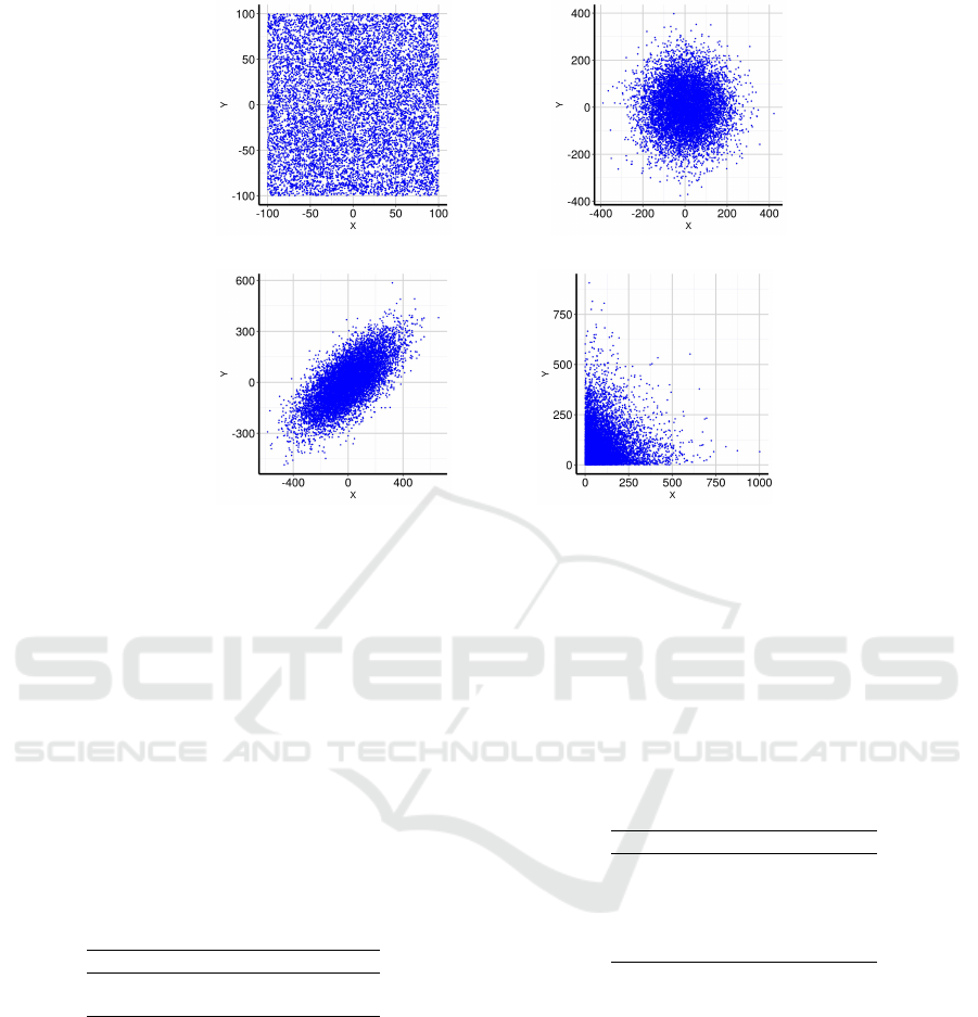
(a) Uniform distribution on a square. (c) Normal distribution.
(d) Bivariate normal distribution. (e) Exponential distribution.
Figure 3: Scatter plots generated using distribution functions.
the uniform distribution. Results of the uniform dis-
tribution are shown in Table 1. The same conclusions
were obtained on all the distributions.
4.3 Test for Homogeneity of Variance
We used the Levene test which is an inferential statis-
tics test used to evaluate the equality of the variances
for a variable calculated for two or more groups (the
most common assessment).
Table 2: Result of the Levene test for groups formed with
the uniform distribution, test used to evaluate the equality
of the variances needed for an ANOVA.
Df F value Pr(>F)
group 19 10.58 0.0000
780
See table 2 where “Df”, “F value” and “Pr(>F)”
respectively correspond to the degrees of freedom, the
value of the test statistic, and the p-value for the test.
The p-values are less than the significance level of
0.05 in all the distributions, which indicates that the
assumption on equality of variances between groups
is not met.
For each case size (for example for 10000 points),
the experiment was repeated 40 times, therefore,
groups are of equal size (40). We can ignore the ho-
mogeneity of variance assumption if we have equal
sample sizes for each group.
4.4 Normality Test
The Shapiro-Wilk test was used for testing normal-
ity in each sample/group. This provides better power
than the Kolmogorov-Smirnov test even after the Lil-
liefors correction (Steinskog et al., 2007).
Table 3: Result of the Shapiro-Wilk test for the groups
formed with the uniform distribution.
Grupo W P.value
1 G010 0.97 0.39
2 G020 0.97 0.40
3 G030 0.96 0.18
···
20 G200 0.98 0.55
There is no enough evidence to conclude that the
assumption of normality in all the distributions is not
met, because the p-values are greater than the signif-
icance level of 0.05. Results of the uniform distribu-
tion are shown in Table 3.
4.5 Empirical Study on the Average
LEPP Size
In this section, we analyze the average LEPP size ob-
tained for the triangulation of each set of vertices, that
is, for randomly generated points with different distri-
bution functions. Groups of vertices of different sizes
were formed, starting with groups of size 10000 and
GRAPP 2020 - 15th International Conference on Computer Graphics Theory and Applications
372

using successive increments of 10000 up to obtain
groups of 200000 points. For each group size (case
size) the experiment was repeated 40 times in order to
obtain general results avoiding non-compliance with
the assumptions of the analysis of variance. Then,
summaries of the means of each group of triangula-
tions, the maximum LEPP, the average LEPP, were
computed.
Table 4: Means obtained for each group of triangulations
formed with the uniform distribution (number of vertices in
thousands).
No.
vertices mTriangles mMax.L mLEPP mSD.L
10 19974.05 11 3.0485 0.0115
20 39971.78 12 3.0512 0.0099
30 59971.50 12 3.0561 0.0075
40 79970.52 12 3.0587 0.0059
50 99969.60 12 3.0590 0.0063
60 119968.73 12 3.0597 0.0057
70 139969.30 13 3.0607 0.0044
80 159967.25 13 3.0619 0.0049
90 179968.05 13 3.0626 0.0043
100 199967.52 13 3.0629 0.0043
110 219967.62 13 3.0637 0.0046
120 239966.98 13 3.0645 0.0037
130 259967.25 13 3.0641 0.0033
140 279967.03 13 3.0648 0.0034
150 299967.65 14 3.0650 0.0034
160 319966.22 13 3.0652 0.0029
170 339965.25 14 3.0662 0.0033
180 359965.83 14 3.0662 0.0030
190 379966.58 14 3.0664 0.0037
200 399965.50 14 3.0661 0.0028
Table 4 presents results of the uniform distribu-
tion. This is composed of 20 rows, each of them
including the summary of the obtained averages for
each group of 40 experiments, which were formed
from a fixed number of vertices in each group. The
column No.vertices indicates the number of vertices
used in each experiment group, the column mTrian-
gles shows the average number of triangles obtained
for the group, while, mMax.L is the average of the
maximum LEPP of the group’s experiment, mLEPP
is the average LEPP size, and mSD.L is the aver-
age of the standard deviations for each group. Note
that the average LEPP size remains almost constant,
in relation to the maximum LEPP size, which in-
creases slightly because each row represents a group
of greater number of vertices.
Figure 4 and 5 show the variability of the aver-
age LEPP size. Note that the variability is greater for
groups formed with less vertices and is reduced when
the number of vertices increases. The same behavior
was obtained for all the distributions.
Figure 4: Scatterplot of the average LEPP in relation with
the number of vertices formed with the uniform distribution.
Figure 5: Box plot of the average LEPP size according to
the number of vertices (groups) - formed with the uniform
distribution.
4.6 Difference of Means Test
The following hypothesis was used to perform the
equality test.
H
0
: all the LEPP means of the groups formed with
the (uniform, normal, normal bivariate, or expo-
nential) distributions are equal.
H
1
: at least one pair of the LEPP means formed
with the (uniform, normal, normal bivariate, or
exponential) distributions are different.
Table 5: Summary result of the analysis of variance for the
difference of means between the groups formed with the
uniform distribution.
Df F value Pr(>F)
Group 19 33.34 0.0000
Residuals 780
In Table 5 we present results on the ANOVA anal-
ysis, Note that for data groups of the uniform distribu-
tion, the p-value is less than the significance level of
0.05, Therefore, the null hypothesis is rejected even
for the significance level of 0.001 and it is concluded
that there is significant difference between the groups.
The same conclusion was obtained for all the distribu-
tions.
Study on the Average Size of the Longest-Edge Propagation Path for Triangulations
373

4.7 One-sample T-test for the Groups of
Vertices Generated According to
Each Probability Distribution
The following hypothesis was used to perform the t
test on each set of vertices.
H
0
: The average LEPP size of the triangulations
constructed from the sets of points generated with
probabilistic distributions is equal to four.
H
1
: The average LEPP size of the triangulations
constructed from the sets of points generated with
probabilistic distributions is less than four.
Table 6: Test t for the vertices of each group and each dis-
tribution (number of vertices in thousands).
No.
vertices
Uniform Normal N.Bivariate Exponential
p-value p-value p-value p-value
10 6.08e-77 9.50e-74 2.53e-77 2.85e-73
20 2.27e-79 2.23e-80 5.38e-85 1.34e-79
30 5.88e-84 9.25e-88 1.05e-82 1.96e-85
···
200 2.65e-100 6.73e-100 2.64e-96 1.00e-94
In Table 6, where the columns represent each dis-
tribution and the rows represent the different groups,
one can see that the p-values are less than the signif-
icance level of 0.05, and the decision is to reject the
null hypothesis. We conclude that the average LEPP
size is significantly less than 4. In the same way, tests
were conducted and it was concluded that the average
LEPP size is significantly greater than 2. Therefore,
the results of the Theorem 2 are empirically and sta-
tistically confirmed (at the significance level of 0.05).
4.8 Regression Analysis
Linear models can be used for prediction or to evalu-
ate whether there is a linear relationship between two
numerical variables (Diez et al., 2015). We have used
linear, quadratic, logistic and logarithmic regressions
to study the data.
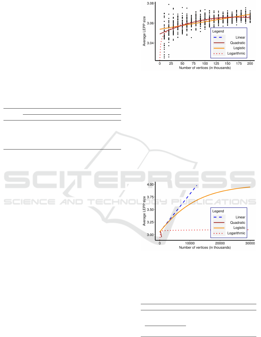
Scatterplot formed with the uniform distribution
and regressions computed on the average LEPP size
with respect to the number vertices, are shown in Fig-
ure 6 (n ≤ 200000). The logistic curve slightly over-
laps the linear one, and Figure 7 clarifies this behavior
(zoom out).
Note that there is a significant relationship between
the average LEPP size and the number of vertices x,
in the four regression models, because the p-values
are much less than 0.05 (significance level) as shown
in Table 7.
The Figures 6 shows a very weak upward trend in
the data, so slight we can hardly notice it. In the lin-
Figure 6: Scatterplot formed with the uniform distribution
and regression models on the average LEPP size with the
number vertices (the logistic curve slightly overlaps the lin-
ear one).
ear regression model, the average LEPP size tends to
grow rapidly and without limit, so it is discarded (see
Figure 7). The quadratic regression attains a maxi-
mum and then decreases producing negative values
when n → ∞, so it is discarded. The logistic regres-
sion model fits well the data and has asymptotic limit
equal to 4 (LEPP=4 as the theory predicts). In ex-
change, the logarithmic regression model has the best
adjusted R squared, that is, it fits the data better in re-
lation to the other models, and keeps well the LEPP
average, as shown in Figures 6 and 7.
Figure 7: Projections of the regression models of the uni-
form distribution (zoom out). The quadratic regression de-
creases and produces negative values when n →∞.
Table 7: Summary of regression model results. First row is
linear regression, second row is quadratic regression, third
row is logistic regression, fourth row is logarithmic regres-
sion.
Regression model for LEPP Adj.R
2
p-value
3.054 +7.535e5x 0.36 1.99e-79
3.049 +0.000205x −6.19e-7x
2
0.42 2.74e-96
4
1 +e
−1.172−0.000104x
0.36 1.57e-79
3.035 +0.0042 log
2
x 0.44 1.42e-102
GRAPP 2020 - 15th International Conference on Computer Graphics Theory and Applications
374

5 CONCLUSIONS
Under an assumption on equal probability for neigh-
bor triangles, we have proven that the average LEPP
size over triangulations of random points sets, is be-
tween 2 and 4 with standard deviation between 0 and
√
6. We also presented a extensive statistical study
over triangulation of random point sets generated with
four distribution functions (uniform, normal, bivariate
normal and exponential), showing that in practice, the
average LEPP size is in agreement with the theory.
Since in computational terms the LEPP cost is con-
stant Θ(1), these results contribute to support LEPP
algorithms and LEPP techniques for triangulation im-
provement in 2-dimensions. More research is needed
to study the distribution of terminal edges in the mesh.
As future research we also suggest to study the av-
erage LEPP size in 3-dimensions, which seems to be-
have analogously to 2-dimensions in practice. This is
a more difficult problem since in 3-dimensions the im-
provement properties of the longest edge bisection of
tetrahedra have not been yet stated. (Rivara and Levin,
1992; Rivara and Palma, 1997).
REFERENCES
Balboa, F., Rodriguez-Moreno, P., and Rivara, M. C.
(2019). Terminal star operations algorithm for tetra-
hedral mesh improvement. In Proceedings 27h Inter-
national Meshing Roundtable, Lecture Notes in Com-
putational Science and Engineering 127, Xexi Roca -
Adrian Loiselle (Eds), Springer Nature Switzeland AG
2019,, 269-284.
Bedregal, C. and Rivara, M. C. (2014a). Longest-edge al-
gorithms for size-optimal refinement of triangulations.
Computer-Aided Des. 46, 246–251.
Bedregal, C. and Rivara, M. C. (2014b). New results
on lepp-delaunay algorithm for quality triangulations.
Procedia Eng. 124, 317–329.
Diez, D., Barr, C., and C¸ etinkaya-Rundel, M. (2015). Open-
Intro Statistics. OpenIntro, Incorporated.
Pion, S. and Yvinec, M. (2019). 2D triangulation data struc-
ture. In CGAL User and Reference Manual. CGAL
Editorial Board, 4.14 edition.
Rivara, M. C. (1984a). Algorithms for refining trian-
gular grids suitable for adaptive and multigrid tech-
niques. International Journal Numerical Methods En-
grg, 20(4), 745-756,.
Rivara, M. C. (1984b). Mesh refinement processes based on
the generalized bisection of simplices. SIAM J. Numer.
Analysis, 21(3), 604-613.
Rivara, M. C. (1997). New longest-edge algorithms for the
refinement and/or improvement of unstructured trian-
gulations. Int. J. Mumer. Methods Eng. 40(18), 3313–
3324.
Rivara, M. C. and Calderon, C. (2010). Lepp terminal
centroid method for quality triangulation. Computer-
Aided Des. 42(1), 58–66.
Rivara, M.-C. and Levin, C. (1992). A 3D refinement al-
gorithm suitable for adaptative and multi-grid tech-
niques. Comunications in Applied Numerical Meth-
ods, 8:281–290.
Rivara, M.-C. and Palma, M. (1997). New LEPP algorithms
for quality polygon and volume triangulation: Imple-
mentation issues and practical behavior. The 1997
Joint ASME/ASCE/SES Summer Meeting. Northwest-
ern University. Evanston Illinois.
Rivara, M. C. and Rodriguez-Moreno, P. (2019). Tuned ter-
minal triangles centroid delaunay algorithm for qual-
ity triangulation. In Proceedings 27h International
Meshing Roundtable, Lecture Notes in Computational
Science and Engineering 127, Xexi Roca -Adrian
Loiselle (Eds), Springer Nature Switzeland AG 2019,
211-228.
Sedgewick, R. and Flajolet, P. (2013). An Introduction to
the Analysis of Algorithms. Pearson Education, 2 edi-
tion.
Sedgewick, R. and Wayne, K. (2011). Algorithms.
Addison-Wesley, 4 edition.
Steinskog, D. J., Tjøstheim, D. B., and Kvamstø, N. G.
(2007). A cautionary note on the use of the
kolmogorov-smirnov test for normality. Monthly
Weather Review, 135:1151–1157.
Thomopoulos, N. T. (2018). Probability Distribu-
tions: With Truncated, Log and Bivariate Extensions.
Springer International, 1 edition.
Vilca, O.-A. (2009). Estudio del refinamiento de mallas
geom
´
etricas de tri
´
angulos rect
´
angulos is
´
osceles. Mas-
ter’s thesis, Departamento de Ciencias de la Com-
putaci
´
on, Santiago - Chile.
Vilca, O.-A., Rivara, M.-C., and Gutierrez, C. (2010).
C
´
alculo de la longitud media de propagaci
´
on del
LEPP. In Proceedings, CSPC-2010, pages 35–42,
Arequipa-Per
´
u. Sociedad Peruana de Computaci
´
on.
Yvinec, M. (2019). 2D triangulation. In CGAL User and
Reference Manual. CGAL Editorial Board, 4.14 edi-
tion.
Study on the Average Size of the Longest-Edge Propagation Path for Triangulations
375