
Twitter Topic Progress Visualization using Micro-clustering
Takako Hashimoto
1
, Akira Kusaba
2
, Dave Shepard
3
, Tetsuji Kuboyama
2
, Kilho Shin
2
and Takeaki Uno
4
1
Chiba University of Commerce, Japan
2
Gakushuin University, Japan
3
University of California, Los Angeles, U.S.A.
4
National Institute of Informatics, Japan
kuboyama@tk.cc.gakushuin.ac.jp, uno@nii.jp
Keywords:
Twitter, Topic Transition Analysis, Micro Clustering, Time Series Analysis.
Abstract:
This paper proposes a method for visualizing the progress of a bursty topic on Twitter using a previously-
proposed micro-clustering technique, which reveals the cause and the progress of a burst. Micro-clustering
can efficiently represent sub-topics of a bursty topic, which allows visualizing transitions between these sub-
topics over time. This process allows for a Twitter user to see the origin of a bursty topic more easily. To show
the method’s effectiveness, we conducted an experiment on a real bursty topic, a controversy over childcare
leave in Japan. When we extract sub-topics using micro-clustering, and analyze micro-clusters over time, we
can understand the progress of the target topic and discover the micro-clusters that caused the burst.
1 INTRODUCTION
It is common for events to produce large amounts of
social media content, both reactions to an event and
comments about various actors in the event. For ex-
ample, in August 2019, a male employee of Kaneka,
a Japanese company, requested leave after the birth of
his child. Shortly after, his company transferred him
to a new division, in apparent retaliation for the re-
quest. When his wife complained about the transfer
on Twitter, a large number of Twitter users tweeted
in support of the employee, which created a PR night-
mare for Kaneka. The company’s poor response to the
situation only worsened their image: they removed
webpages describing their leave policies, and argued
that their decision to transfer the man was justified.
Such decisions only worsened their image in the pub-
lic eye, and produced even more negative tweets.
As in the case of the Kaneka employee, one large
overarching topic really consists of many small sub-
topics, and it is possible to focus on one of the small
sub-topics and lose sight of the overarching topic.
Awareness of the many topics, and which serves as the
origin of the other topics, is essential to understanding
all facets of a topic. For example, when companies
attempt to handle negative PR, they need to be aware
of the original actions that triggered a negative public
image, and later actions that improve or worsen their
image.
Automatic topic transition detection has been a
major area of research for the last ten years. Conven-
tional methods based on latent topic extraction from
high dimensional vector spaces such as LDA(Blei
et al., 2003) can extract major topics, but operate pri-
marily with coarsely-grained topics. Even versions
of these methods modified to handle time series data
are often too coarse to capture the emergence of these
topics over time, or how individual users react to
them. Conventional approaches focusing on tweets
with specific keywords can analyze topics over time,
but provide little insight into how people react to a
topic.
Our previous work proposed a method for ana-
lyzing topic transition using micro-clustering, an ap-
proach that creates clusters smaller than those created
by conventional clustering methods(Hashimoto et al.,
2019a). Building on that work, this paper proposes
a method for understanding the progress of topics on
Twitter. The novel contribution of this paper is to pro-
pose a visualization method for analyzing the transi-
tion of micro-clusters from tweets in each topic in a
time series. This is a sort of ”review process” that
allows a human reader to examine a bursty topic. In
our method(Hashimoto et al., 2019a), micro-clusters
Hashimoto, T., Kusaba, A., Shepard, D., Kuboyama, T., Shin, K. and Uno, T.
Twitter Topic Progress Visualization using Micro-clustering.
DOI: 10.5220/0009160805850592
In Proceedings of the 9th International Conference on Pattern Recognition Applications and Methods (ICPRAM 2020), pages 585-592
ISBN: 978-989-758-397-1; ISSN: 2184-4313
Copyright
c
2022 by SCITEPRESS – Science and Technology Publications, Lda. All rights reserved
585

are extracted by our original technique (Uno et al.,
2015; Uno et al., 2017) from millions of tweets. Each
micro-cluster represents sub-topics such as diverse
opinions about the topic, or smaller events within
a larger event. After extracting micro-clustesrs, we
observe each micro-cluster’s rise and fall over time,
and therefore, topic transitions. Bursts emerge when
many users tweet about a specific topic. Some offline
behaviors accelerate the burst. Detecting the behav-
iors that cause the burst helps understand its origin,
and can be useful for managing future actions.
2 RELATED WORK
Time series topic analysis targeting social media has
become an active area of research. One type of ap-
proach uses word co-occurrence to track topic tran-
sition over time(Jin et al., 2017)(Kwak et al., 2010).
These methods are useful for extracting dominant top-
ics, but they do not have a fine enough resolution to
distinguish subtle but important differences between,
for example, a real and a fake subtopics, or differ-
ences among incompatible opinions in a topic. It is
also difficult to extract a small amount of representa-
tive keywords showing the topic content.
A number of methods have been proposed to
track topic transitions over time based on conven-
tional topic extraction methods such as LDA and
LSA. In these methods, topics are extracted on each
window in a time series, and connected according
to their similarities to track their transitions (Kitada
et al., 2015; Fujino and Hoshino, 2014; Wang et al.,
2012). These methods characterize clusters with a set
of keywords based on word occurrences, and high-
frequency words tend to be extracted as keywords.
Time-series LDA is, in fact, an active area of re-
search (Yeh et al., 2016; Jaradat and Matskin, 2019).
However, topics in LDA are often coarsely-grained;
LDA cannot produce a topic model with a large num-
ber of topics in a reasonable amount of time. Our
method addresses these limitations because it works
with finer-grained topics and does not involve train-
ing a model through Gibbs sampling.
We can extract keywords using conventional
methods, but it is more difficult to make sense of
them, since these conventional methods extract a few
big clusters and many small clusters. A method such
as TopicSketch(Xie et al., 2016) is one example: Top-
icSketch can handle high volumes of time series data
efficiently, but the topics it produces are coarsely
grained and bursty. This one, and similar methods,
do not work well for producing a detailed picture of
a large, complex topic because they tend to put small
but interesting subtopics into one big topic. For exam-
ple, if a rumor emerges as part of a larger topic, con-
ventional methods will often produce a single topic
about that rumor. However, while a rumor is circu-
lating, there will be people retweeting the rumor, peo-
ple commenting on the rumor, and people questioning
that rumor. A conventional topic modeling method
would group all of these into that one topic. Our
method produces finer-grained topics which would
separate each of these into their own clusters.
Regarding TopicSketch specifically, our method
has two additional advantages. First, it is simpler to
implement. Second, it would likely not be as vul-
nerable to the manipulations that the TopicSketch au-
thors mention, which is that a spammer could cre-
ate the illusion of interest in a topic. If a spammer
were attempting, for example, to promote a music
album, the spammer could inject a large number of
tweets with the same content about that album. Our
method would isolate those tweets into their own clus-
ter, which would make them easier to filter out.
To address these problems, we propose an effi-
cient method for detecting time series topic transition
by micro-clustering. Especially in this paper, we pro-
pose the visualization method to analyze the transition
of micro-clusters from tweets in each topic in a time
series.
3 PROPOSED METHOD
Our basic technique was explained in our previous
work(Hashimoto et al., 2019a; Hashimoto et al.,
2019b). This section briefly explains our technique,
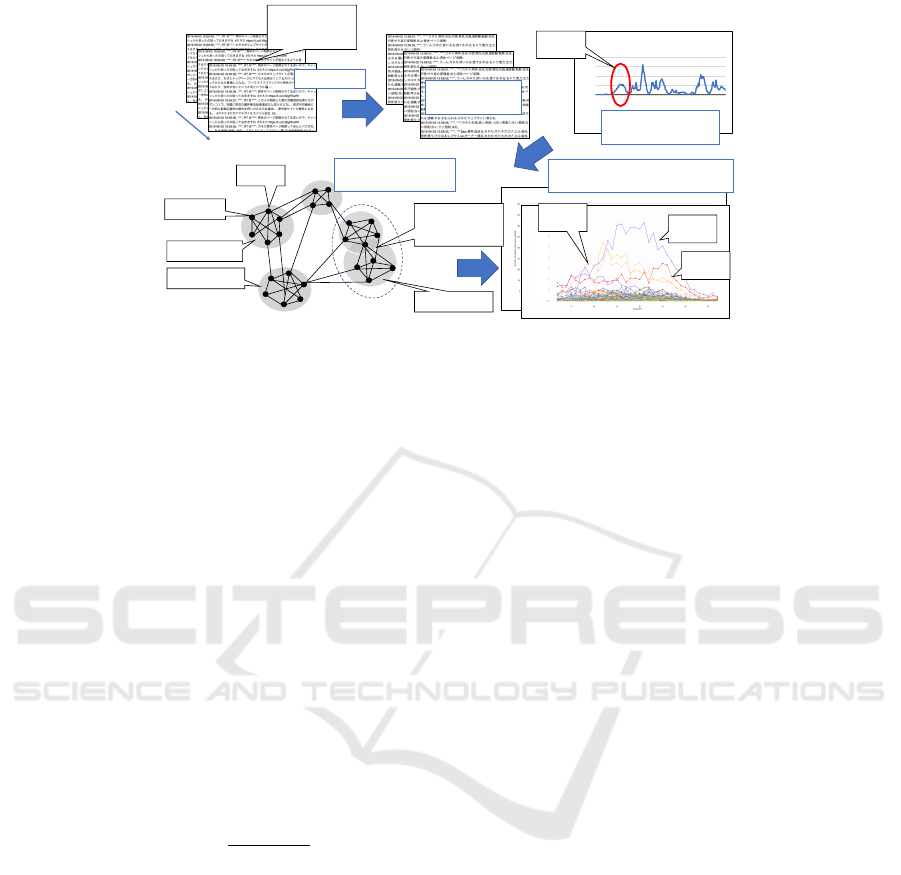
before introducing our new contribution: a visualiza-
tion method for these topics that helps to detect the
cause of the overarching topic (Figure 1).
3.1 Input Data and Morphological
Analysis
First, we gather data by collecting tweets that in-
clude certain keywords. As the input data (A), we
group the tweets sequentially into fixed-length win-
dows (e.g. half an hour) based on their times-
tamps. We then create the sequence of tweet
id
-word
id
count matrices (B) using a morphological analysis
technique, hTW
0
, TW
1
. . . , TW
t
, . . . , TW
T
i that con-
tains the words used in each tweet during each time
period. To segment tweets that may not have used
spaces to delineate word boundaries, we employed
the Japanese morphological analyzer, MeCab (Kudo,
2006). These time series matrices, TW
0
, . . . , TW
T
, are
obviously sparse.
ICPRAM 2020 - 9th International Conference on Pattern Recognition Applications and Methods
586
7K
C
CEBD
-A-
K
K
3DAKD
CB9K
4EB
-
0
1
4EB
4EB
--
7KE
L99D
KDEK
&--
#
###
###
###
###
##(8 8 #
##(8 8 #
##)#8 #8 ##
##)#8 #8 #
##)#8 8 ##
##)#8 #8 #
##)#8 #8 ##
##)#8 #8 #
##)#8 )8 ##
##)#8 8 #
##)#8 #(8 ##
##)#8 8 #
##)#8 8 ##
##)#(8 ##8 #
##)#(8 #8 ##
##)#(8 8 #
##)#(8 #8 ##
##)#)8 #8 #
##)#)8 #8 ##
##)#)8 (8 #
##)#)8 8 ##
##)#8 #8 #
##)#8 8 ##
##)#8 8 #
7K5C
-
-
2LKE
7C
6
E7K
4E
B
4E
B
4E
B
Figure 1: Proposed Method.
3.2 Tweet Counts Over Time
Then we count the number of tweets in each time slot.
The graph (C) shows the progress of the number of
tweets about the target topic. If the topic becomes
popular, it should have several bursts. We explore
the bursts sequentially, since earlier bursts may cause
later bursts.
3.3 Graph Generation
Next, a similarity graph of tweets (D) is formed dur-
ing the burst. In the graph, each tweet tw
i
in TW
t
is
a node. Next, tweets that have similar words are con-
nected by edges. To evaluate tweet similarity, we use
the Jaccard coefficient (Jaccard, 1912), a measure for
comparing the similarity of sets.
J(tw
i
, tw
j
) =
tw
i
∩ tw
j
tw
i
∪ tw
j
We set the threshold s. If the Jaccard coefficient
between nodes is larger than s, we add an edge be-
tween these nodes. By changing the threshold s, we
can control the form of the graph. A smaller s will
produce a graph with more edges, while a larger s will
produce a graph with fewer edges.
3.4 Micro-clustering using Data
Polishing
Our method uses a data polishing algorithm for
micro-clustering (D) (Uno et al., 2015; Uno et al.,
2017). This section describes the data polishing al-
gorithm briefly; for more information, please see the
cited papers (Uno et al., 2015; Uno et al., 2017).
Micro-clusters are groups of data records that are re-
lated, but do not overlap. A set of micro-clusters
should satisfy the following conditions:
1. Quantity (the number of micro-clusters found
should not be huge)
2. Independence (micro-clusters should not be simi-
lar)
3. Coverage (all micro-clusters should be found)
4. Granularity (the granularity of micro-clusters
should be the same)
5. Rigidity (the micro-clusters found should not
change because of non-essential changes such as
random seeds or indices of records)
In a graph, micro-clusters correspond to dense
subgraphs, and non-edges in the dense subgraphs are
ambiguities. The procedure for data polishing for
micro-clustering involves adding edges for these non-
edges, and removing these ambiguous edges from the
graph. Data polishing is emphasizing the structure
by adding and removing edges. For identifying these
non-edges and edges, we consider the following fea-
sible hypothesis. If nodes u and v are in the same
clique of size k, u and v have at least k − 2 common
neighbors. A clique is a subset of vertices of a graph
such that every two distinct vertices in the clique are
adjacent. Thus, we have
|
N[u] ∩ N[v]
|
≥ k, and this
is a necessary condition that u and v are in a clique
of size at least k. We call this condition k-common
neighbor condition. If u and v are in a sufficiently
large pseudo clique, they are also expected to satisfy
this condition. In contrast, if two nodes do not sat-
isfy the condition, they belong to a pseudo clique with
very small probability. Even though they belong to a
pseudo clique, they actually seem disconnected in the
clique. Thus we may decide that they should not be
Twitter Topic Progress Visualization using Micro-clustering
587

in the same cluster. Let P
k
(G) = (V, E
0
) where E
0
is
the collection of edges connecting node pairs satisfy-
ing the k-common neighbor condition, and the pol-
ishing process is the computation of P
k
(G) from G.
We call this process k-intersection polishing. To eval-
uate k-common neighbor condition, we also use the
Jaccard coefficient. We set the threshold s
0
and if the
Jaccard coefficient between nodes u and v considering
their neighbors is larger than s
0
, the edge is generated
between them. Maximal clique enumeration is per-
formed using an algorithm such as MACE(Sch
¨
utze
et al., 2008). By changing the threshold s
0
, we can
control the micro-clustering. If the threshold s is
smaller, the each micro-cluster tends to be larger and
if the threshold s
0
is larger, each micro-cluster tends
to be smaller.
The graph after micro-clustering adaptation (D)
shows sub-topics of the first burst. Each micro-cluster
is considered a sub-topic during the first burst of the
target topic.
3.5 Time Series Visualization for the
Specific Burst
Then we count the number of tweets of each micro-
cluster over time (E) during the target burst. In Figure
1 (E), the horizontal axis shows the time slots of the
target burst, and the vertical axis shows the number of
tweets of each micro-cluster that were posted at each
time slot. The threshold s and s
0
that were explained in
Section 3.3 and 3.4 respectively control the granular-
ity of micro-clusters. The graph shows the sub-topic
growth. Through the visualization, we can understand
the progress of the topic during the target burst, and
infer the cause of the burst.
4 EXPERIMENTAL RESULT
We conducted the experiment with NYSOL Python
(NYSOL Corporation, ), a library for big data. All
the experiments were conducted on a MacBook Pro
wiht a 2.7 GHz Intel Core i7 processor and 16GB of
RAM.
4.1 Target Topic
Our target topic is the reaction to a controversy over
a Japanese company’s childcare leave policy, which
arose on Twitter in early June 2019. The following
are the major events in the target topic:
• January, 2019: A woman gave birth
• March, 2019: Her husband took childcare leave
• April, 2019: The husband returned to work
• May, 2019: The husband’s company informed
him that he would be transferred
• June 1, 2019: The wife tweeted a complaint about
her husband’s transfer. Many Twitter users ex-
pressed their support for the woman and criticized
the company.
• June 1, 2019: The company removed their web
pages about childcare leave
• June 3, 2019: The company posted a press release
arguing that the wife’s post was wrong, and at-
tempting to justify their decision to transfer the
man
• June 6, 2019: The company posted another press
release attemping to justify their decision
4.2 Input Data and Morphological
Analysis
We built a dataset by crawling tweets that included the
company name ”Kaneka” from 08:00:00 on May 29
to 00:29:59 on June 8, harvesting a total of 192,393
tweets. This dataset offers a significant document of
users’ responses to the target topic. These tweets were
grouped in 30-minute windows, producing a time se-
ries of 465 slots. Then we applied the morphological
analysis technique to tweets in each time slot.
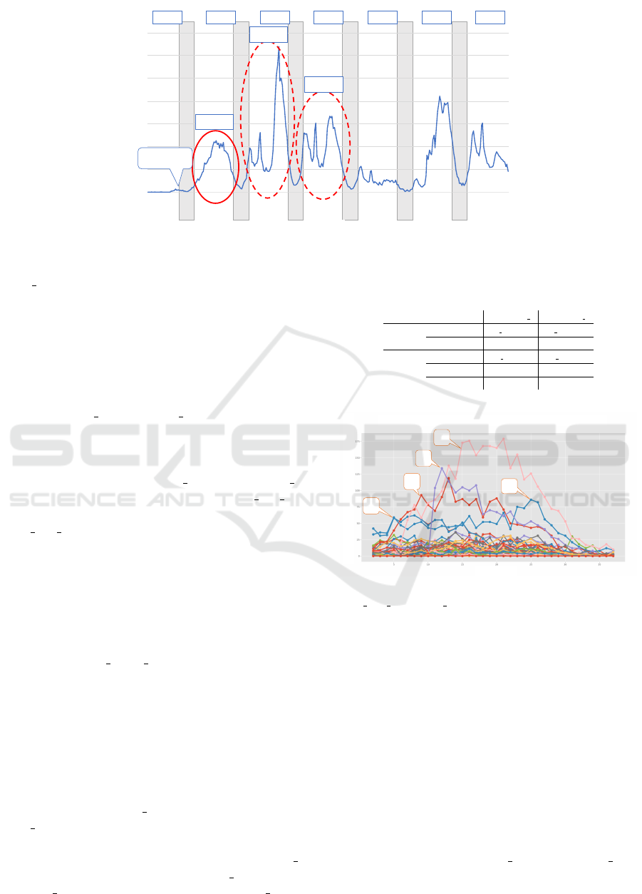
4.3 Count of Number of Tweets Over
Time
Figure 2 shows the number of tweets harvested in
each time slot. After the wife tweeted her com-
plaints, the topic burst started. Then, several more
bursts happened after the wife’s tweet. From the num-
ber of tweets posted, it is clear that the topic con-
tinued to attract attention on Twitter, but why? We
use our method to analyze the burst. As the first step,
we analyze the first burst (Burst1), which consists of
24,839 tweets posted during June 1 21:00:00 - June 2
18:59:59 (22 hours).
4.4 Graph Generation
In this experiment, we did not distinguish be-
tween tweets and retweets. We conducted two sub-
experiments with the parameter values shown in Ta-
ble 1 to show how our method can extract micro-
clusters with different granularities based on the
thresholds s and s
0
, which are explained in Section
3.3 and 3.4 respectively. To form a similarity graph,
we set the Jaccard coefficient thresholds to s 1 = 0.5
ICPRAM 2020 - 9th International Conference on Pattern Recognition Applications and Methods
588
#
#
0 #0 #
# 0 #0 #
#0 0
#0 0 #
0 0
0 0
0 0
0 0
0 0
0 0
0 0
0 0
0 0
0 0
0 0
0 0
0 0
0 0
#0 0
#0 0
#0 0
#0 0
#0 0
#0 0
#0 0
#0 0
#0 0
#0 0
#0 0
#0 0
0 0
0 0
0 0
0 0
0 0
0 0
0 0
0 0
0 0
0 0
0 0
0 0
0 0
0 0
0 0
0 0
0 0
0 0
0 0
0 0
0 0
0 0
0 0
0 0
0 0
0 0
0 0
0 0
0 0
0 0
0 0
0 0
0 0
0 0
0 0
0 0
0 0
0 0
0 0
0 0
0 0
0 0
0 0
0 0
0 0
0 0
0 0
0 0
115
61 61 61# 61 61 61 61
35147
7211
61
321911
89
89
89#
Figure 2: # of Tweets in Each Time Slot.
and s 2 = 0.3, with values derived from experimenta-
tion. The threshold s = 0.5 is stricter, and produces
a clearer structure that consists of similar tweets, but
it might miss semantically-similar tweets that express
the same idea using slightly different wording. If we
set the threshold s < 0.3, we find too many tweet
pairs that use a couple of the same words to express
dissimilar ideas. Therefore, we empirically decided
the thresholds s
1 = 0.5 and s 2 = 0.3. As the first
step, we formed the graphs based on the similarity of
tweets in the Burst1 of Figure 2.
Table 1 shows the threshold parameters and the
number of edges of Experiment 1 and Experiment 2.
Namely, the number of edges for Experiment 1 (s 1 =
0.5) is larger than the number of edges for Experi-
ment 2 (s 2 = 0.3).
4.5 Micro-clustering using Data
Polishing
Next, we use data polishing to form micro-clusters
from the Burst1 of Figure 2. We set the Jaccard coef-
ficient threshold s
0
1 = s
0
2 = 0.2 through experimen-
tation. Our tests showed that values 0.1 < s
0
<= 0.4
make little difference in the result. If we set a thresh-
old s
0
<= 0.1, the method creates micro-clusters that
are too large; if we set a threshold s
0
>= 0.5, the
method produces too many small clusters. We then
add edges between nodes that have similar neighbor
sets. Table 1 shows the parameters.
Data polishing increases the numbers of edges to
10,094,803 (Experiment
1) and 35,153,218 (Experi-
ment 2) respectively. Finally, we performed maximal
clique (M-Clique) enumeration. M-Clique enumera-
tion produced 708 maximal cliques in Experiment 1
and 597 maximal cliques in Experiment 2. Since Ex-
periment 2 has more edges than Experiment 1, the
Table 1: Parameters, # of Edges, and # of Maximal Cliques
in the Experiment for the Burst1 (24,839 tweets).
Experiment 1 Experiment 2
Similarity s s 1 = 0.5 s 2 = 0.3
Graph # of Edges 9,853,981 21,657,803
Data s’ s’ 1 = 0.2 s’ 2 = 0.2
Polishing # of Edges 10,094,803 35,153,218
Graph # of MCliques 708 597
-3
34-3333:1332
1 3C532:53B33:
#
Figure 3: Micro-Clusters’ Progress during Burst1: Experi-
ment 1 (s 1 = 0.5, s’ 2 = 0.2).
size of micro-clusters tends to be larger, while the
number of M-Cliques became smaller.
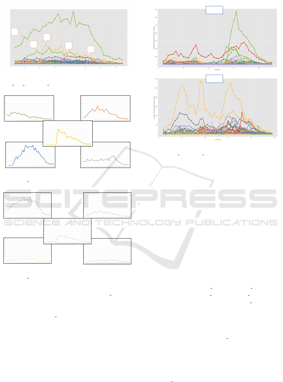
4.6 Time Series Visualization on a
Specific Burst
Next, we count the number of tweets in each micro-
cluster during the target burst (E). In Figure 3 and
4, the horizontal axis shows the time slots during
Burst1, and the vertical axis shows the number of
tweets posted at each time slot. By adjusting the
threshold s and s
0
, we can control the granularity of
micro-clusters. Figure 3 is more granular than Fig-
ure 4, because the threshold s
1 is larger than s 2. A
larger threshold s creates edges between more similar
tweets. Data polishing generates tighter
Twitter Topic Progress Visualization using Micro-clustering
589
-3
34-3333:1332
1 3C532:53B33:
#
Figure 4: Micro-Clusters’ Progress during Burst1: Experi-
ment 2 (s 2 = 0.3, s’ 2 = 0.2).
#
Figure 5: Top 5 Micro-Clusters’ Progress during Burst1:
Experiment 1.
#
Figure 6: Top 5 Micro-Clusters’ Progress during Burst1:
Experiment 2.
micro-clusters. Therefore, the threshold s 1(= 0.5)
produces more clusters, which shows the progress of
the target burst in more detail (Figure 3). On the other
hand, the threshold s 2(= 0.3) produces fewer clus-
ters, which shows less detail (Figure 4).
We extract major micro-clusters that have large
number of tweets from Figure 3. From Figure 3, the
top five micro-clusters are extracted(Figure 5). Each
cluster shows a unique pattern of change over time.
Micro-cluster #1 occurs at the beginning of the burst
and gradually disappears. Micro-cluster #2 peaks dur-
ing the early part of the burst. #3 is special: it sud-
denly occurs and gradually declines. #4 is the biggest
one, and shows a typical burst. #5 is stable. It has
almost the same number of tweets in the period.
Burst2
Burst3
Figure 7: Micro-Clusters’ Progress during the Burst2 and
the Burst3 (s 1 = 0.5, s’ 2 = 0.2).
Table 2 shows the major tweets of micro-clusters
#1-#5 and a description of their contents. #1 consists
of a debate over Kaneka’s authorization for childcare
support by the Japanese Health and Welfare Ministry.
This is a straightforward reaction to the wife’s tweet.
#2 contains messages about the deletion of the com-
pany’s childcare leave page on the web. #3 discusses
the deletion of the company’s childcare leave page,
but also mentions the fact that a backup copy of the
page could be found on another site. Obviously, users
only showed interest in this topic once the copy was
created. #4’s and #5’s tweets make up the majority
of the burst. Both micro-clusters consist mainly of
tweets criticizing the company’s decision. Figure 5
shows that #2, #3 and #4 are the cause of the burst of
the larger overall topic.
Because Experiment 2’s threshold s 2(= 0.3) is
smaller than Experiment 1’s threshold s 1(= 0.5), the
number of micro-clusters in Experiment 2 is smaller.
Micro-clusters in Figure 4 are less granular. Table 3
shows more larger micro-clusters than Table 2. From
Figure 4, we also extract the top five micro-clusters.
In Figure 6, the biggest micro-cluster #1 consists of
#1, #4, and #5 of Experiment 1. Thus, the biggest
micro-cluster #1 in Figure 6 is the micro-cluster that
includes tweets criticizing the company. #2 and #3 in
Figure 6 are related to the deletion of the company’s
childcare leave page. #4 and #5 micro-clusters in Fig-
ure 6 also contain criticism of Kaneka. Even in Ex-
periment 2, micro-clusters related to the deletion of
Kaneka’s childcare leave page are still generated. The
deletion of childcare leave page is the most significant
ICPRAM 2020 - 9th International Conference on Pattern Recognition Applications and Methods
590

Table 2: Major Tweets and Contents of Top Five Micro-
Clusters of Burst1: Experiment 1 (s 1 = 0.5, s’ 2 = 0.2).
ID Major Tweets Contents
1 Kaneka was authorized as a child-rearing
support company by the the Health and
Welfare Ministry. I can’t believe it. We
cannot trust the authorization. Kaneka bul-
lies employees.
This micro-cluster shows the
beginning of condemnation for
Kaneka.
2 The page for childcare leave has been
deleted, so I’ll post it from the cache.
This micro-cluster contains
tweets about the deletion of
childcare pages from Kaneka’s
website.
3 Kaneka deleted the childcare leave pages,
because Twitter erupted with a post about
a male employee who has taken childcare
leave.
This micro-cluster directs us to
the site containing an archived
version of the deleted childcare
pages from Kaneka’s website.
4 I personally think that it is not his childcare
leave but his home building. There are a lot
of employees who were forced to leave the
house just after their home was completed.
Apparently it’s just after a mortgage, so it’s
likely that he won’t quit even if he makes a
violent personnel change.
This micro-cluster suggests
another reason for the com-
pany’s decision: construction
of his home.
5 I think that there are some old Japanese
companies that used excuses like “trans-
ferred when he bought a house” and “trans-
ferred when a child was born”. The era
has definitely changed since things will
be spread by SNS. Kaneka should be de-
feated.
This micro-cluster shows con-
demnation of Kaneka’s deci-
sion to transfer the employee.
Table 3: Major Tweets and Contents of Top Five Micro-
Clusters of Burst1: Experiment 2 (s 2 = 0.3, s’ 2 = 0.2).
ID Major Tweets Contents
1 I personally think that it is not his childcare
leave but his home building. There are a lot
of employees who were forced to leave the
house just after their home was completed.
Apparently it’s just after a mortgage, so it’s
likely that he won’t quit even if he make a
violent personnel change.
This micro-cluster is a com-
bined cluster consists of #1, #4
and #5 of Figure refF6.
2 The page for childcare leave has been
deleted, so I’ll post it from the cache.
This micro-cluster is also
related to the deletion of
childcare pages from Kaneka’s
website.
3 Kaneka deleted the childcare leave pages,
because Twitter erupted with a post about
a male employee who has taken childcare
leave.
This micro-cluster directs us
to a site containing an archive
of the deleted childcare pages
from Kaneka’s website.
4 It is a retirement issue due to forced trans-
fer, but if you are a shareholder, it is very
bad.
This micro-cluster examines
another reason for the com-
pany’s decision. It was not the
childcare leave, but his home
building.
5 Moreover, it is a clear violation of the law
not to allow paid vacation use. It is also
a violation for the company to specify the
retirement date. Even my previous job
(SMEs close to black) was paid when I quit
...
This micro-cluster is a com-
bined cluster for the condem-
nation for Kaneka’s decision
related to the transfer. Posters
are worries about the stock
price.
event in this burst.
For Burst2 and Burst3 in Figure 2, micro-
clustering can be adopted as well (Figure 7). To an-
alyze the micro-clusters in Figure 7, we detect the
causes of the burst.
5 CONCLUSION
This paper proposed a visualization method for ex-
amining bursting Twitter topics based on micro-
clustering. The finer degree of detail offered
by micro-clustering makes the differences between
users’ reactions clearer by subdividing those reactions
into subtopics. Evaluating micro-clusters over time
allows us to identify the causes of a target burst topic.
In our future work, we intend to apply our method
to different topics about a greater variety of events.
We also plan to propose a model for detecting topic
bursts in social media automatically.
ACKNOWLEDGEMENTS
This work was partially supported by JSPS KAK-
ENHI Grant Numbers 18K11443, 19K12125,
19H01133, 19J00871, and 17H00762.
REFERENCES
Blei, D. M., Ng, A. Y., and Jordan, M. I. (2003). Latent
dirichlet allocation. Journal of machine Learning re-
search, 3(Jan):993–1022.
Fujino, I. and Hoshino, Y. (2014). A method for identifying
topics in twitter and its application for analyzing the
transition of topics. In Proc. of DEIM 2014, C4-2.
Hashimoto, T., Uno, T., Kuboyama, T., Shin, K., and Shep-
ard, D. (2019a). Time series topic transition based on
micro-clustering. In 2019 IEEE International Confer-
ence on Big Data and Smart Computing (BigComp),
pages 1–8. IEEE.
Hashimoto, T., Uno, T., Kuboyama, T., Shin, K., and Shep-
ard, D. (2019b). Time series topic transition based on
micro-clustering. In 2019 IEEE International Confer-
ence on Big Data and Smart Computing (BigComp),
pages 1–8. IEEE.
Jaccard, P. (1912). The distribution of the flora in the alpine
zone. 1. New phytologist, 11(2):37–50.
Jaradat, S. and Matskin, M. (2019). On dynamic topic mod-
els for mining social media. In Emerging Research
Challenges and Opportunities in Computational So-
cial Network Analysis and Mining, pages 209–230.
Springer.
Jin, H., Toyoda, M., and Yoshinaga, N. (2017). Can cross-
lingual information cascades be predicted on twitter?
In International Conference on Social Informatics,
pages 457–472. Springer.
Kitada, T., Kazama, K., Toriumi, T. S. F., Kurihara, A.,
Shinoda, K., Noda, I., and Saito, K. (2015). Analysis
and visualization of topic series using tweets in great
east japan earthquake. In The 29th Annual Confer-
ence of the Japanese Society for Artificial Intelligence,
2B3-NFC-02a-1.
Kudo, T. (2006). Mecab: Yet another part-of-speech and
morphological analyzer. http://mecab. sourceforge. jp.
Kwak, H., Lee, C., Park, H., and Moon, S. (2010). What
is twitter, a social network or a news media? In
Proceedings of the 19th international conference on
World wide web, pages 591–600. AcM.
Twitter Topic Progress Visualization using Micro-clustering
591

NYSOL Corporation. NYSOL. https://www.nysol.jp/.
Sch
¨
utze, H., Manning, C. D., and Raghavan, P. (2008). In-
troduction to information retrieval. In Proceedings
of the international communication of association for
computing machinery conference, page 260.
Uno, T., Maegawa, H., Nakahara, T., Hamuro, Y., Yoshi-
naka, R., and Tatsuta, M. (2015). Micro-clustering:
Finding small clusters in large diversity. arXiv
preprint arXiv:1507.03067.
Uno, T., Maegawa, H., Nakahara, T., Hamuro, Y., Yoshi-
naka, R., and Tatsuta, M. (2017). Micro-clustering
by data polishing. In 2017 IEEE International Con-
ference on Big Data (Big Data), pages 1012–1018.
IEEE.
Wang, Y., Agichtein, E., and Benzi, M. (2012). Tm-lda:
efficient online modeling of latent topic transitions
in social media. In Proceedings of the 18th ACM
SIGKDD international conference on Knowledge dis-
covery and data mining, pages 123–131. ACM.
Xie, W., Zhu, F., Jiang, J., Lim, E.-P., and Wang, K. (2016).
Topicsketch: Real-time bursty topic detection from
twitter. IEEE Transactions on Knowledge and Data
Engineering, 28(8):2216–2229.
Yeh, J.-F., Tan, Y.-S., and Lee, C.-H. (2016). Topic detec-
tion and tracking for conversational content by using
conceptual dynamic latent dirichlet allocation. Neuro-
computing, 216:310–318.
ICPRAM 2020 - 9th International Conference on Pattern Recognition Applications and Methods
592
