An Optimization Method for a Multi-day Distribution Problem with

Shortage Supplies

Netiphan Amphaiphan

and Wasakorn Laesanklang

1,2

Department of Mathematics, Faculty of Science, Mahidol University, Rama VI Road,

Ratchathewi, Bangkok, 10400, Thailand

Centre of Excellence in Mathematics, CHE, Thailand

Keywords:

Multi-period Vehicle Routing Problem, Shortage Supplies, Distribution, Mixed Integer Programming Model.

Abstract:

We investigated a multi-day distribution problem while supplies are limited. This scenario can be found

in post-natural disasters or economic crisis such as ﬂoods, earthquakes, palm oil shortage crisis, etc. The

objective function of this problem is to minimize total traveling distance, unsatisﬁed cost, and variance of

supply delivery proportion. In order to solve this multi-day problem optimally, it requires large computing

memory and takes a long computational time. Therefore, we divided these large problems into multiple daily

sub-problems and solved the sub-problems with the exact method. The sub-problems were solved sequentially

for which the prior daily sub-problem is to be tackle ﬁrst and the following daily sub-problems are deﬁned

based on the prior daily sub-problem solution. Changes were applied to update demands and to adjust delivery

priority. There are three delivery priority setups proposing in this paper. Also, we present an experiment using

the three proposed methods to solve modiﬁed Solomon’s vehicle routing problem datasets which extended a

single period vehicle routing problem with time windows to be seven-day routing problems.

1 INTRODUCTION

This paper proposes an exact-heuristic hybrid method

to solve a multi-day distribution problem with short-

age supplies. Normally, supply distribution in normal

situation is an operation which has been studied for

many years. The problem has been shown in many

paper and text books such as N-location distribution

problem (Karmarkar and Patel, 1977) and produc-

tion distribution problem (Boudia et al., 2007). How-

ever, there are situations where supplies are limited in

which a normal distribution operation is not practical

because there are too many demands that cannot be

ﬁlled. Supplies shortages are not normally occur in

high or medium income countries. Although, emer-

gency and disaster situations may cause the supply

shortages. For example, in 2011, Thailand encoun-

tered an extreme ﬂood triggered by Tropical Storm

Nock-Ten. There were 13.6 million people stuck

in the disaster area. Thai government transformed

government buildings, schools, university buildings

to be temporally shelters because majority of houses

were unable to occupied. People in these relieve care

needed food, medicine and other supplies so that they

could survive the day. Meanwhile, these commodi-

ties could not reproduce in the disaster area, they were

transported from other part of Thailand to a distribu-

tion center. The operation at distribution center was

indeed challenging as it must ﬁll demands in remote

area, at which might not have road access. In some

case, the operation may have a limitation due to the

number of vehicles and their capacity rather than a

limitation of supplies. Recently, in 2019, there was

another tropical storm hit the northeastern of Thai-

land. There were reports of insufﬁcient relieve goods

and distribution problem in post-disaster event. This

has shown that there were no efﬁcient plan to deal

with the distribution problem with limited supplies in

Thailand.

An example of the real-life supply shortages were

the case when Thailand faced the palm oil crisis in

2011. Palm oil production was decrease and there

were no supplies in the market. An immediate policy,

which was order from the Thai government to limit

palm oil purchase per transaction to three liters. The

policy applies in order to prevent consumer to stock-

pile palm oil. Similarly, distributor cannot apply nor-

mal distribution operation because the best possible

solution is to have the palm oil products to sell near

distribution center. This plan will indeed effect cus-

356

Amphaiphan, N. and Laesanklang, W.

An Optimization Method for a Multi-day Distribution Problem with Shortage Supplies.

DOI: 10.5220/0009154703560363

In Proceedings of the 9th International Conference on Operations Research and Enterprise Systems (ICORES 2020), pages 356-363

ISBN: 978-989-758-396-4; ISSN: 2184-4372

tomers who live very far from the distribution center

that they cannot have excess to the product in a rea-

sonable price. Therefore, these rare events needs a

special operation plan.

This paper proposes a method to ﬁnd supply dis-

tribution plan especially when all demands cannot be

fulﬁlled. The solution of this problem gives a plan

to distribute supplies with one vehicle mode in multi-

ple periods. The plan should ration supplies equally

among the demand points. We present a mathematical

programming model for a multi-day distribution prob-

lem with shortage supplies. However, this model can-

not be solved as our sample problems are very com-

putationally expensive. Therefore, we implement a

method utilizing a mixed integer programming model

to tackle this problem by solving the problem in a

daily basis and to have demand information passing to

the next day problem to balance supplies distribution.

The goal is to generate routing plans for the whole

time period and to have an equal supply distribution.

The remaining of the paper is organized as fol-

lows. We discuss related research in Section 2. Sec-

tion 3 describes the problem and its assumptions.

It also present our weekly quadratic programming

model. Section 4 gives a daily problem and how our

plan is recalculated. Section 5 describes the dataset

used in this work and the results from our method.

Section 6 presents our conclusions.

2 LITERATURE REVIEW

There were several literature for transportation prob-

lem in post natural disasters. (

Ozdamar et al., 2004)

proposed a model that generated an emergency logis-

tic plan for natural disaster. They investigated a sce-

nario when supplies were limited and there were pre-

diction of demands. (Liu et al., 2007) studied large-

scale emergency plans and proposed a mathematical

model to minimize the total unsatisﬁed demands. (Af-

shar and Haghani, 2012) developed a comprehensive

model for pick up and delivery schedule for natu-

ral disasters. (Hsueh et al., 2008) studied a vehicle

routing problem for disasters with two-phase deci-

sions, tactical decisions and routing decisions. (He

and Zhang, 2016) determined priority allocation co-

efﬁcient for post-disaster relief supplies using set the-

ory. (Qin et al., 2017) investigated insufﬁcient emer-

gency supplies in the initial period right after a dis-

aster event with uncertain demands of affected loca-

tions. This proposed solution method was split into

two stages, determining the serviced demand point

and optimizing the related factors such as a number of

used vehicles, supplies and routes. (Liu et al., 2019)

studied a location-routing problem for the early post-

earthquake where relief goods were insufﬁcient. The

goal was to ﬁnd a fair distribution plan using a de-

mand loss function.

Emergencies and disasters mainly create short

term insufﬁcient supply situations. However, there

were researches dealing with long term supply short-

ages such as a distribution problem with limited in-

ventory (Chien et al., 1989) and blood supply chain

in Thailand (Chaiwuttisak et al., 2014).

There were many ways to solve large-scale prob-

lems such as local search, neighborhood search, ge-

netic algorithm, etc. Problem decomposition is a

technique that can be applied to make a large prob-

lem become smaller sub-problem so that the solver

ﬁnd a solution faster. (Kim and Kim, 1999) decom-

posed a multi-period vehicle scheduling problem into

N single-retailer problems to generate delivery sched-

ule. (Cheng and Wang, 2009) investigated VRP with

time window constraints using decomposition tech-

nique to reduce the problem size. (Laesanklang and

Landa-Silva, 2017) also applied decomposition and

repair methods for home healthcare planning to ob-

tain a feasible solution.

There were a few research works in the litera-

ture tackled multi-period supplies shortage problem

such as blood supply chain in Thailand (Chaiwutti-

sak et al., 2014) and multi-depot production planning

(Parthanadee and Logendran, 2006). The studies on

general multi-period VRP with shortage supplies are

relatively rare. Our work investigates a multi-period

VRP with supply shortages while splitting the prob-

lem into multiple daily sub-problems.

3 MULTI-DAY DISTRIBUTION

WITH SHORTAGE SUPPLIES

This section describes the quadratic programming

model for the multi-day distribution problem with

shortage supplies. The problem is to generate a trans-

portation plan over a multi-day period with supply

shortage event. Therefore, solutions for this trans-

portation plan should distribute the products equally

to all demand nodes. This may differ from the normal

distribution operation for which it is to ﬁnd the min-

imum operation cost. The assumptions for the multi-

day distribution problem with shortage supplies are

listed below.

1. Transportation costs and travel times are propor-

tional to travel distances. Also, transportation cost

from any location i to j in all periods are identical.

2. Distance from location i to location j equals to

An Optimization Method for a Multi-day Distribution Problem with Shortage Supplies

357

distance from location j to location i.

3. Each customer must be visited no more than once

a day.

4. The total delivered commodities must not exceed

vehicle capacity.

5. Each location must be visited no more than once

per day but that visit may have not ﬁll the demand

in full.

6. All vehicles are homogeneous.

7. Demands are given for all locations for the whole

time horizon. Although, demands may accumu-

late if the demand point has not been visited.

Ideally, to have the best possible solution, the multi-

day problem should be solved as a whole. We may

present this problem using a quadratic programming

model.

3.1 Weekly Problem

As we mentioned in Section 1, we would like to ﬁnd

delivery plans that have equally supply distribution

for every demand node. Therefore, the quadratic pro-

gramming model was proposed for this problem.

Table 1 presents notations to be used in this paper.

The notations can be grouped as sets, parameters, and

variables.

The decision is to assign a set of vehicles V to

make visit at a set of locations C at time period in a set

of time T. Each vehicle v ∈ V has maximum capacity

and each location i ∈ C also has demands on day

t ∈ T , represented by s

. We considered a distribution

with single depot so that c

and c

are artiﬁcial start

and end nodes where the two artiﬁcial nodes represent

one physical depot.

The problem is constructed based on graph where

nodes or vertices are locations to visit and the edges

are routes between the two locations. A variable x

v,t

i,l

a binary decision variable in which x

v,t

i,l

= 1 represents

that a vehicle v must make a visit at location l after

location i at day t, and x

v,t

i,l

= 0 otherwise. An assign-

ment to travel between location i and location j has

corresponding distance d

i, j

and travel time α

i, j

. Also,

an integer variable δ

v,t

is the arrival time of the vehi-

cle v ∈ V at location i ∈ C on day t ∈ T . y

is a binary

decision variable where its value is 1 when no vehicle

make visit at location i ∈ C on day t ∈ T , and y

= 0

indicates otherwise. A variable p

v,t

is a variable be-

tween 0 to 1 for determining delivery proportion. In

this problem, it is possible to delivery partial demands

as the supplies are very limited and rationing must

be enforce to distribute the commodity equally for all

Table 1: Notations for the multi-day distribution problem

with shortage supplies.

Sets

C A set of locations.

V A set of vehicles.

T A set of time period. ( T = {1, 2, ..., 7})

Parameters

i, j

Distance between node i and j.

M Penalty cost of not assigning visit a node.

i, j

Travel time from node i to j.

Weight for each location i at time t.

Vehicle capacity of vehicle v

Demand of location i on day t

A weight associated to total transportation cost.

A weight associated to unsatisﬁed cost.

A weight associated to variance of

proportion of delivered supply.

Variables

v,t

i, j

Binary decision variable with value 1 indicating

that vehicle v is assigned to visit i and then

move to visit j on day t, and 0 otherwise.

Binary decision variable with value of 1

indicating that visit i on day t is unassigned,

and 0 otherwise.

v,t

Arrival time at node i assigned to vehicle v

on day t

v,t

Delivery proportion delivered to customer i by

vehicle v on day t (0 ≤ p

v,t

≤ 1)

demand points. Therefore, we deﬁne β

as the pro-

portion of delivered supplies and the total demands at

location i for the whole time horizon. This proportion

can be written as

∑

t∈T

∑

v∈V

v,t

· s

∑

t∈T

In order to measure equal distribution, we then mini-

mize the variance of β

. Note that we use

β as a nota-

tion of an average of all β

From the above notation, we present the mathe-

matical model for the multi-day distribution problem

with shortage supplies below.

Min. ω

∑

t∈T

∑

i, j∈C

∑

v∈V

i, j

· x

v,t

i, j

+ ω

∑

t∈T

∑

i∈C

∑

v∈V

− s

· p

v,t

)

+ ω

∑

j∈C

(β

−

β)

|C|

(1)

ICORES 2020 - 9th International Conference on Operations Research and Enterprise Systems

358

Subject to

∑

v∈V

∑

i∈C∪{c

}

v,t

i,l

+ y

= 1 ∀l ∈ C, t ∈ T (2)

∑

i∈C∪{c

}

v,t

= 1 ∀v ∈ V, t ∈ T (3)

∑

i∈C∪{c

}

v,t

i,c

= 1 ∀v ∈ V, t ∈ T (4)

∑

i∈C∪{c

}

v,t

i,r

∑

j∈C∪{c

}

v,t

r, j

∀v ∈ V, r ∈ C, t ∈ T (5)

∑

i∈C

· p

v,t

≤ q

∀v ∈ V, t ∈ T (6)

∑

i∈C∪{c

}

v,t

i, j

≥ p

v,t

∀v ∈ V, j ∈ C, t ∈ T (7)

∑

i∈C∪{c

}

v,t

i, j

≤ M · p

v,t

∀v ∈ V, j ∈ C, t ∈ T (8)

· p

v,t

≥ 0.05 · q

· x

v,t

i, j

∀v ∈ V, i, j ∈ C ∪ {c

}, t ∈ T

(9)

v,t

i, j

+ x

v,t

j,i

≤ 1 ∀v ∈ V, i, j ∈ C, i 6= j, t ∈ T (10)

v,t

+α

i, j

−(1−x

v,t

i, j

)·M ≤ δ

v,t

∀v ∈ V, i ∈C∪{c

j ∈ C ∪ {c

}, i 6= j, t ∈ T (11)

The objective function of the proposed multi-day dis-

tribution with shortage supplies is to minimize a sum-

mation of three weighted costs (1). The ﬁrst cost is the

total travelling distances for the whole time horizon.

The second cost is the unsatisﬁed cost, which is mea-

sured from the number of accumulated demands that

have not been served at the end of the time horizon.

The third cost is to have equal supply distribution,

which is measured by the percentage of delivered sup-

ply variance. The percentage delivered supply vari-

ance is to measure differences between delivery pro-

portion, in which the ideal solution should be the case

where all locations get the same proportion of supply

or the delivery proportion variance should equal to 0.

Therefore, the proposed model is to minimising the

percentage supply variance should provide a fair dis-

tribution plan. There are corresponding weights to the

above objective function costs which are ω

, ω

, and

, respectively.

We set the variance as the highest priority to min-

imize. Hence, the weight ω

is the highest in this

objective function. The second priority is to mini-

mize the cost of unsatisﬁed demands where the cor-

responding weight is ω

. The lowest priority is to

minimize the cost of travelling distances, where the

weight is ω

. We followed weight parameter setting

from (Rasmussen et al., 2012). These weights are set

by ω

= 1, ω

∑

i∈B

∑

j∈B

i, j

and ω

= ω

|C| max

i∈C,t∈T

The proposed mathematical model has the follow-

ing constraints to complete the multi-day distribution

problem with shortage supplies. First, constraint (2)

ensures that a visit l ∈ C is either assigned to a ve-

hicle v ∈ V by having one of x

v,t

i,l

= 1 or left unas-

signed by having y

= 1 for every time period t ∈ T .

For each day, a vehicle must leave a depot from con-

straint (3) and it must return to depot at the end of

the day (4). During the day, a vehicle must travel to

visit a list of locations, where the ﬂow conservation

constraint guarantees the condition such that a vehi-

cle v arrives at a location l, it must leave that location

(5). Constraint (6) deﬁnes maximum vehicle capacity

for which the total delivery must not exceed. Con-

straints (7) and (8) control that the p

v,t

can be more

than 0 only if the sum of x

v,t

i, j

is 1. Furthermore, a visit

to be made must delivery supplies at least 5 % of the

vehicle capacity. Constraint (10) prevents vehicle v to

return to a location i ∈C if it has been left the location.

Constraint (11) is a sub-tour elimination constraint in-

dicating that the arrival time at location j ∈ C must be

more than the arrival time at location i ∈ C, given that

the vehicle v ∈ V must visit location j after location i

v,t

i, j

= 1) (Moshref-Javadi and Lee, 2016).

The mathematical programming model for the

multi-day distribution problem with shortage supplies

above is a quadratic programming model as it ap-

plies variance as one of the objective function. The

problem is a np-hard so that applying exact method

to solve this problem may not be the best approach.

Therefore, we propose a method to sequentially solve

daily sub-problems using a mixed integer program-

ming model and mathematical solver to tackle this

problem.

4 SOLUTION METHOD

This section explains our proposed method to solve

the multi-day distribution problem with shortage sup-

plies. We formulate a MIP model for a daily problem

and use it to solve the multi-day problem. The multi-

day problem is then split into multiple daily problems.

Each daily problem is then solved by the exact solver

to get the best solution with a limited computation

time. A next day problem is then updated with de-

mands and historical supplies to adjust the next day

delivery plan.

Algorithm 1 illustrates the steps of our proposed

method. A multi-period vehicle routing problem can

be denoted by P = (V, B), where V is the set of ve-

hicles and B is the set of locations. The goal is to

assign vehicles to make visits at multiple locations

within the time horizon. Our proposed method has

An Optimization Method for a Multi-day Distribution Problem with Shortage Supplies

359

three steps, which are decomposing problem, solving

sub-problems and updating parameters. At the updat-

ing parameter step, demands and delivery priority of

a problem at period t depend on the solution of the

problem at period t − 1. This step allows us to solve

the problem as a day-by-day in sequential basis. The

updating parameter step is the key to balance the sup-

ply delivery.

Algorithm 1: Algorithm for solution method.

Data: Problem P=(V,B), V is the set of

vehicles and B is the set of all

locations

Result: {SolutionPath} sub sol

1 begin

2 {Problem} T=ProblemDecomposition

(V,B);

3 SortSubProblem(t);

4 for day t ∈ T do

5 sub sol (t)=cplex.solve (t, s

, γ

);

6 Update data (d

, γ

);

7 end

8 end

4.1 Problem Decomposition

Our proposed method tackles this problem in a day-

by-day basis. Therefore, we split this one week

problem into seven daily sub-problems. These sub-

problems will be solved sequentially, such that the

sub-problem at period t will be processed before the

sub-problem at period t + 1. Structure of each sub-

problem is identical with the full problem such that

it has a set of vehicles and a set of locations with all

constraints applied.

The daily sub-problems will be formulated as a

mixed integer programming model and to be solved

by a mathematical solver.

4.2 Daily Sub-problem

We implement a mixed integer programming model

for the daily sub-problems. Originally, our multi-day

problem is a quadratic programming problem as it

is required to have balance supply distribution. In

this daily problem, we re-implement the quadratic

term into linear factor. Hence, we replace the term

∑

j∈C

(β

−

β)

|C|

with a weighted delivered demands γ

· p

v,t

. To balance delivery priority, we use weight

adjustment step which will be explained in the next

subsection.

Therefore, mixed integer programming model for

the daily problem is presented below. Note that at

time period t

∈ T , all variables are considered at time

Min.

∑

i, j∈C∪{c

}

∑

v∈V

i, j

· x

v,t

i, j

∑

i∈C

M ·y

−

∑

v∈V

∑

j∈C

· s

· p

v,t

(12)

Subject to

∑

v∈V

∑

i∈C∪{c

}

v,t

i, j

+ y

= 1 ∀ j ∈ C (13)

∑

j∈C∪{c

}

v,t

, j

= 1 ∀v ∈ V (14)

∑

i∈C∪{c

}

v,t

i,c

= 1 ∀v ∈ V (15)

∑

i∈C∪{c

}

v,t

i,r

∑

j∈C∪{c

}

v,t

r, j

∀v ∈ V, r ∈ C (16)

∑

j∈C

× p

v,t

≤ q

∀v ∈ V (17)

∑

i∈C∪{c

}

v,t

i, j

≥ p

v,t

∀v ∈ V, j ∈ C (18)

∑

i∈C∪{c

}

v,t

i, j

≤ M · p

v,t

∀v ∈ V, j ∈ C (19)

· p

v,t

≥ 0.05 ·v

· x

v,t

i, j

∀v ∈ V, i ∈ C ∪ {c

}, j ∈ C

(20)

v,t

i, j

+ x

v,t

j,i

≤ 1 ∀v ∈ V, i, j ∈ C, i 6= j (21)

v,t

+ α

i, j

− (1 − x

v,t

i, j

) · M ≤ δ

v,t

∀v ∈ V,

i ∈ C ∪{c

}, j ∈ C ∪ {c

}, i 6= j (22)

4.3 Updating Parameters

Updating parameter step is to balance delivery distri-

bution. The problem assumption does not require that

all locations have to be visited in one day, but visits

may distribute for the whole horizon. For one day

plan, it is possible that some locations left unassigned

or some locations may be visited but they are received

partial demands.

Table 2 presents settings for γ

parameter. The

parameter sets delivery priority for which the assign-

ments should prioritise a visit j over the other visits at

day t when the visit has the highest γ

. In this paper,

we propose three parameter settings. The ﬁrst setting

is the case where the γ

remains the same for every

time period. The second setting is to double the prior-

ity value to locations that have not been visited in the

time period t − 1. The third setting is to double the

ICORES 2020 - 9th International Conference on Operations Research and Enterprise Systems

360

Table 2: Three setups for changing weight of locations.

Setup Description

1 γ

= γ

t−1

for all locations.

2 γ

= 2γ

t−1

for all locations that have not

been visited on day t −1.

3 γ

= 2γ

t−1

for some locations that have

not been visited on day t −1.

priority value for some locations that have not been

visited on day t −1.

For all these cases, we assume that their demands

are accumulated if the needs have not been delivered.

Therefore, the demand parameter is to be changed by

= d

t−1

+ d

t−1

· (1 − p

v,t−1

). For example, location

a has ordered 10 units of product every day. On the

ﬁrst day, this location may receive the commodity for

6 units. Thus, on day 2, the location a may request

this product for another 10 units. Hence, an updated

demand for location a on day 2 is equal to 10+(10-

6)=14.

The method was implemented in JAVA with a

well-known commercial mathematical solver, IBM

ILOG CPLEX Optimization Studio (CPLEX) in a

process to solve the daily MIP model.

5 EXPERIMENTS AND

COMPUTATIONAL RESULTS

In this section, we explain our modiﬁed datasets, ex-

perimental setups and results of the experiment.

5.1 Datasets

We use modiﬁed Solomon’s datasets in our experi-

ment. The datasets have three instance types which

are randomly generated type (R), clustered type (C),

and mixed type (RC). Originally, Solomon’s datasets

are created for a single period vehicle routing prob-

lem with time windows. The objective function of the

original datasets are to ﬁnd a routing plan which has

the lowest number of assigned vehicles and the short-

est total travel distances. The constraints of the orig-

inal problem are vehicle capacity, delivery time win-

dows and the demands for each location which every

location must be served.

In our modiﬁed Solomon’s dataset, a single pe-

riod VRPTW is expanded to be a seven-day schedul-

ing problem. There are four instances for each origi-

nal dataset type. Each new instance has 25 visit loca-

tions and the original demands are requested repeat-

edly for seven days. The modiﬁed problems do not

require delivery time window, in which the delivery

can be made anytime in a day. Therefore, we created

12 modiﬁed seven-day instances for our experiment.

We also set initial location visiting priority randomly,

which had range between 1 to 3.

5.2 Results

In this section, we present results from our experi-

ments. This experiment compared solutions of the

modiﬁed Solomon’s datasets which obtained from the

proposed algorithm. We set the computational time to

return the best feasible solution if the daily computa-

tional time exceed ﬁve minutes. Thus, the maximum

computation times for a weekly problem is 35 min-

utes.

Table 3 presents objective values of solutions from

three visiting priority setups. Each setup in the ta-

ble presents four objective values, which are total

travel distance (Distance), unsatisﬁed cost (Unsat-

isﬁed), supply distribution variance (Variance), and

the total weekly cost (Weekly cost). There are 12

modiﬁed Solomon’s instances presented in the table.

Bold texts in the table present the best objective value

among the three setups.

Consider the number of the cheapest weekly cost

solutions, there are 3, 2, and 7 best solutions from

Setup 1, Setup 2, and Setup 3, respectively. The

weighted summation of objective values shows that

the unsatisﬁed cost is the most inﬂuential value, fol-

lowed by the percentage of delivered supply variance,

and the total travel distance.

We analyze the result based on the original

Solomon’s dataset types which are randomly gener-

ated dataset (R), clustered generated dataset (C), and

mixed generated dataset (RC).

For dataset type R, Setup 3 provided the best over-

all solutions, in which the Setup 3 found the lowest

weekly cost solutions for three instances. The main

contribution was that the Setup 3 had the lowest over-

all unsatisﬁed delivery plan. Setup 1 provided one

solution with the lowest weekly cost. Also, Setup 1

had the lowest travel distances for every solution for

this dataset type. On the other hand, Setup 2 did not

ﬁnd the best solution and had the highest weekly cost.

For data type C, Setup 2 had the best solution for

two instances when comparing the weekly cost while

Setup 1 and Setup 3 had the best solution for one in-

stance for each setup. Setup 3 also had solution with

the shortest distance for three instances.

For data type RC, Setup 3 provided the minimum

unsatisﬁed cost, variance and weekly cost of three

datasets. Setup 1 and Setup 2 had two solutions pro-

viding the shortest distances. From the result, Setup 2

An Optimization Method for a Multi-day Distribution Problem with Shortage Supplies

361

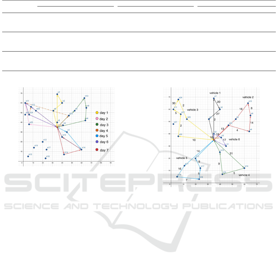
Table 3: Solution weighted costs for the modiﬁed Solomon’s Dataset.

Setup 1 Setup 2 Setup 3

Datasets Distance Unsatisﬁed Variance Weekly cost Distance Unsatisﬁed Variance Weekly cost Distance Unsatisﬁed Variance Weekly cost

Dataset 1-Type R 3,717 5,257,411 39,755 5,300,883 3,789 6,519,331 53,007 6,576,127 3,999 4,849,787 26,504 4,880,290

Dataset 2-Type R 3,751 11,555,526 92,762 11,652,039 4,709 12,321,124 92,762 12,418,595 4,036 11,780,452 92,762 11,877,251

Dataset 3-Type R 3,465 8,486,067 66,259 8,555,791 4,058 8,170,676 79,511 8,254,244 4,091 7,094,634 53,007 7,151,732

Dataset 4-Type R 2,670 9,910,719 66,259 9,979,648 3,467 11,361,697 106,014 11,471,178 3,042 9,741,450 119,266 9,863,757

Dataset 1-Type C 2,510 19,648,281 159,021 19,809,813 2,460 19,660,473 145,769 19,808,702 2,320 19,682,029 172,273 19,856,622

Dataset 2-Type C 2,276 12,176,945 119,266 12,298,487 2,760 13,080,714 106,014 13,189,488 2,627 12,211,753 92,762 12,307,142

Dataset 3-Type C 3,482 24,555,669 172,273 24,731,424 3,445 24,554,433 172,273 24,730,150 3,393 24,610,267 172,273 24,785,932

Dataset 4-Type C 3,791 18,510,574 145,769 18,660,135 3,696 19,305,326 145,769 19,454,791 3,595 18,402,617 145,769 18,551,981

Dataset 1-Type RC 3,603 29,517,301 185,525 29,706,428 3,636 29,551,403 198,776 29,753,815 4,789 29,610,417 172,273 29,787,479

Dataset 2-Type RC 4,550 18,110,902 159,021 18,274,473 4,554 17,572,174 159,021 17,735,749 4,899 15,971,893 145,769 16,122,561

Dataset 3-Type RC 3,779 6,944,624 66,259 7,014,661 3,560 6,980,138 66,259 7,049,957 3,625 6,907,342 66,259 6,977,226

Dataset 4-Type RC 3,504 12,491,983 92,762 12,588,249 3,468 13,007,388 106,014 13,116,870 3,551 12,118,460 145,769 12,267,781

where ω

= 1, ω

= 17669 and ω

= 1325175

Remark: Bold texts present the best objective value among the three setups.

Figure 1: A routing plan of vehicle 1 for dataset 2 type R.

did not perform well when considered weekly costs,

unsatisﬁed demands and supply distribution variance.

Overall, Setup 3 found solutions with the lowest

weekly cost, which contributed from low unsatisﬁed

demands and delivered supply variance. Setup 1 had

the shortest total distance.

As we mention that we preferred a solution with

equal supplies distribution. From this view, we can

conclude that Setup 3 is the best setup because it pro-

vided the best solution for seven instances. From Ta-

ble 3, we recommended that the dataset type R should

be solved by applying Setup 1 because it provides the

best overall costs. Next, we present a solution from

using Setup 1 to solve Dataset 2-Type R.

Figure 1 illustrates a 7-day vehicle scheduling so-

lution for vehicle 1 applying setup 1 to solve Dataset

2-Type R. The instance has 25 visiting locations and

one service depot. There are six vehicles, each has

capacity of 50 units. From the ﬁgure, vehicle 1 is de-

ployed every day. There are locations where the vehi-

cle has visited multiple days such as a path from lo-

cation n

to location n

and return to depot on day 5

and day 7. The solution also shows the case where the

visiting order may not so efﬁcient in term of travelling

distances, such as a route on day 1 (yellow path). This

is because the sub-problem solution is not the optimal

solution because the mathematical solver reaches the

Figure 2: A routing plan of all vehicles on the ﬁrst period

using Setup 1.

computation time limit.

Figure 2 displays a one-day plan of all vehicles.

Each line represents a vehicle path to delivery com-

modities. Numbers on each line represent the number

of commodity to delivery at destination location. For

example, the plan for vehicle 5 is to delivery 14 units

at location n

, 16 units at location n

, 7 units at lo-

cation n

, 5 units at location n

, 8 units at location

and return to depot. From this one-day plan, six

vehicles make visits to 24 locations and only one lo-

cation, n

, has not been visited on day 1. The plan to

visit location n

is on day 3 and day 6.

6 CONCLUSIONS AND FUTURE

WORK

This paper explains a multi-day distribution problem

while supplies are shortage or there are transporta-

tion difﬁculties limiting supply delivery. The aim is

to build visiting plans having fair supply distribution

over planning horizon. We assume a constant de-

mand from every location every day, which then accu-

ICORES 2020 - 9th International Conference on Operations Research and Enterprise Systems

362

mulated with unsatisfactory demands from previous

days.

We propose a hybrid heuristic method to tackle

this multi-day problem as multiple daily sub-

problems. Each sub-problem was solved by a mixed-

integer programming model. We applied heuristic de-

livery priority distribution, so that the locations that

had not been visited on previous days had higher vis-

iting priority. There were three priority distribution

setups applied in our experiment, which were dou-

ble the priority every locations that had not been vis-

ited, double the priority for some locations that had

not been visited, and no priority changes as a control

group. We tested our proposed method with 12 mod-

iﬁed Solomon’s instances.

Our future works includes expanding problem

cases, improving the current algorithm and exploring

other solution approaches. To expand problem cases,

we may added due date and time window constraints

can be included as our future works. It is necessary to

improve the current algorithm to obtain an optimal so-

lution. Our proposed algorithm can also be improved

to tackle larger problems. Also, our future works will

apply other heuristic methods to this problem, such

as neighbourhood search, genetic algorithm, and con-

structive heuristic methods to compare results with

this hybrid heuristic approach.

ACKNOWLEDGEMENTS

We would like to thank Science Achievement Schol-

arship of Thailand (SAST) for ﬁnancial support.

REFERENCES

Afshar, A. and Haghani, A. (2012). Modeling integrated

supply chain logistics in real-time large-scale disaster

relief operations. Socio-Economic Planning Sciences,

46(4):327–338.

Boudia, M., Louly, M. A. O., and Prins, C. (2007). A

reactive grasp and path relinking for a combined

production–distribution problem. Computers & Op-

erations Research, 34(11):3402–3419.

Chaiwuttisak, P., Smith, H., Wu, Y., and Potts, C. (2014).

Blood supply chain with insufﬁcient supply: a case

study of location and routing in thailand. Lecture

Notes in Management Science, 6:23–31.

Cheng, C.-B. and Wang, K.-P. (2009). Solving a vehicle

routing problem with time windows by a decomposi-

tion technique and a genetic algorithm. Expert Sys-

tems with Applications, 36(4):7758–7763.

Chien, T. W., Balakrishnan, A., and Wong, R. T. (1989).

An integrated inventory allocation and vehicle routing

problem. Transportation science, 23(2):67–76.

He, S. and Zhang, L. (2016). Location-routing model

for post-disaster initial stage relief supplies based on

priority level. Chemical Engineering Transactions,

51:973–978.

Hsueh, C.-F., Chen, H.-K., and Chou, H.-W. (2008). Dy-

namic vehicle routing for relief logistics in natural dis-

asters. In Vehicle routing problem. IntechOpen.

Karmarkar, U. S. and Patel, N. R. (1977). The one-period,

n-location distribution problem. Naval Research Lo-

gistics Quarterly, 24(4):559–575.

Kim, J.-U. and Kim, Y.-D. (1999). A decomposition ap-

proach to a multi-period vehicle scheduling problem.

Omega, 27(4):421–430.

Laesanklang, W. and Landa-Silva, D. (2017). Decomposi-

tion techniques with mixed integer programming and

heuristics for home healthcare planning. Annals of

Operations Research, 256(1):93–127.

Liu, C., Kou, G., Peng, Y., and Alsaadi, F. E. (2019).

Location-routing problem for relief distribution in the

early post-earthquake stage from the perspective of

fairness. Sustainability, 11(12):3420.

Liu, D., Han, J., and Zhu, J. (2007). Vehicle routing for

medical supplies in large-scale emergencies. Lecture

Notes in Operations Research, 8:412–419.

Moshref-Javadi, M. and Lee, S. (2016). The customer-

centric, multi-commodity vehicle routing problem

with split delivery. Expert Systems with Applications,

56:335–348.

Ozdamar, L., Ekinci, E., and K

uc¸

ukyazici, B. (2004). Emer-

gency logistics planning in natural disasters. Annals of

operations research, 129(1-4):217–245.

Parthanadee, P. and Logendran, R. (2006). Periodic product

distribution from multi-depots under limited supplies.

Iie Transactions, 38(11):1009–1026.

Qin, J., Ye, Y., Cheng, B.-r., Zhao, X., and Ni, L. (2017).

The emergency vehicle routing problem with uncer-

tain demand under sustainability environments. Sus-

tainability, 9(2):288.

Rasmussen, M. S., Justesen, T., Dohn, A., and Larsen, J.

(2012). The home care crew scheduling problem:

Preference-based visit clustering and temporal depen-

dencies. European Journal of Operational Research,

219(3):598–610.

An Optimization Method for a Multi-day Distribution Problem with Shortage Supplies

363